The Starting Point

Prologue

Alright, let’s get technical. As I’ve mentioned, we’re going to start off with most of the fundamentals someone needs. This post is relatively lengthy and has a few major sections but I’ve decided to keep all of this in one post, rather than two since they’re related. It’s going to be many shallow dips into various topics — mostly computer systems at first, and algorithm terminology at the end.

The rough philosophy revolving around how I’ve structured this post as well as designed the scope is based on the following reasons:

It pays to know a little bit about how algorithms are executed on machines. Ultimately, we need a model that mimics what we expect to happen in real life and without some peek into how modern machines work we have no basis to build a model for.
The depth of each topic I’m covering is limited because I only plan on giving rough context — just enough ground that surrounds and is outside of algorithms. Most courses in algorithms will rarely provide this information and I think as a consequence it often (and easily) leads to misunderstandings about a few key concepts. By doing this I hope to avoid leading to such an issue. The tradeoff, of course, is that before we formally begin talking about algorithms, you need to go through a really thick post on all this prerequisite knowledge.
(Mostly an elaboration of point 1 and 2). I think with a better understanding of a bigger picture, we can make better informed discussions about what is reasonable and what is not. Often times, formal courses do not do this because they are constrained by the time frame of a semester or two. We have the luxury of taking our time to not only cover things, but explain why we are doing what we are doing, and to question the validity of the reasons themselves. This is not so important for beginners, but my grand plan for you, dear reader, is eventually grow into someone who sees and appreciates algorithms the way that I do. And for that, a healthy dose of philosophy is needed every now and then.

An Aside About Models

Author’s Note: If you already know what modeling means (and not the kind with cameras and you ending up on the cover of a magazine), you can safely skip this subsection. If you’re not familiar with what it is, I suggest you stick around because this motivates, pretty much, the entire post.

Some of you might have heard the classic joke in economics:

Economists Do It With Models …because there’s no shortage of demand for curves that they supply.

Whatever underlying nuance aside (yes I’m here to kill that joke by explaining it), a huge part of their job is to try to frame every day occurences in the context of well… many things (like money or social behaviour) in a mathematical context. They might try to turn “happiness” into a number, and then, with a few assumptions about how an equation might decently reflect real life, try to explain why people behave the way they do.

Let’s try doing it for ourselves by considering the Prisoner’s Dilemma. If you’re not familiar with the story, it goes like this:

Two suspects are being interrogated in separate rooms, and each has a choice of betraying the other. If they both choose to keep silent, both will get a year in prison. If one betrays the other who chooses to keep silent, the betrayer will leave scott-free whereas the silent one gets 10 years in prison. If both prisoners betray each other, they both get 3 years in prison.

Now this problem sounds slightly relatable to a real life scenario, doesn’t it? Or at least, it sounds like something that might happen in real life. The incredible part is that one can model this in a mathematical way, and use that to explain why (under the model itself) both would reasonably betray the other person.

Let’s try doing that. We’re going to take it so that the number of years directly correlates to how much of a penalty each suspect receives. Based on that, we can make the following table:

drawing

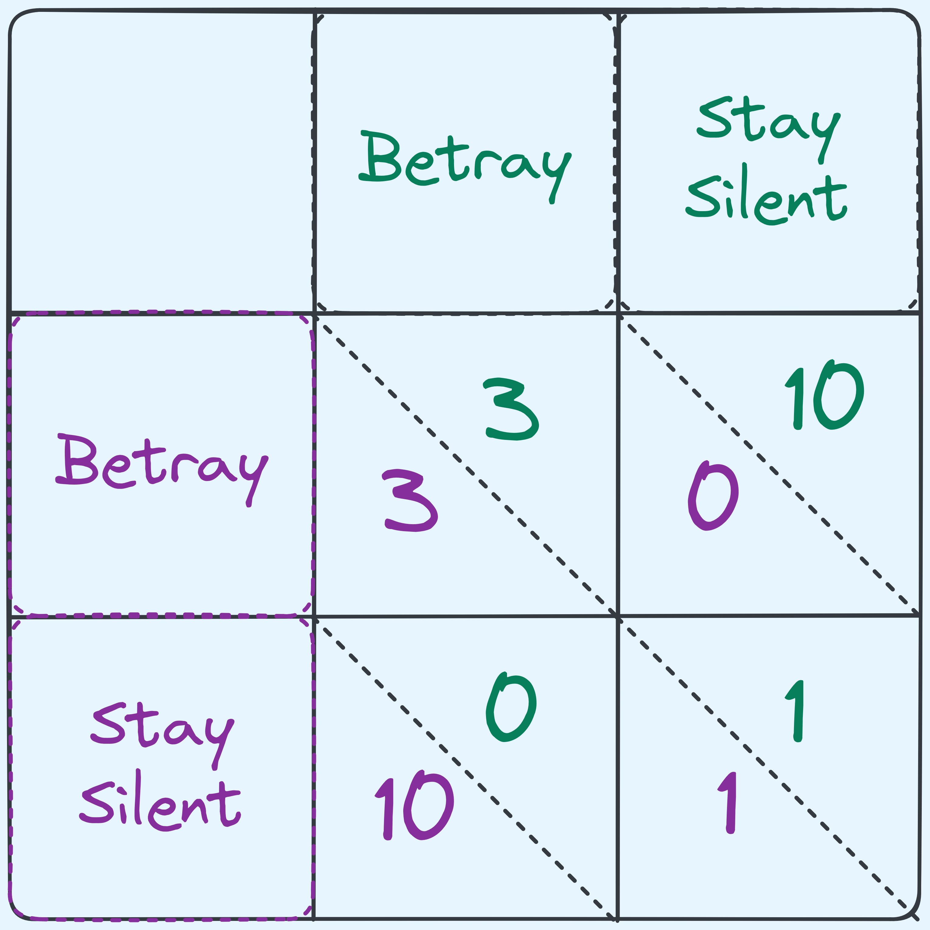
A table that shows the penalties for either suspect.

Now notice that for the green suspect, regardless of what the purple suspect does, he can always reduce their penalty by choosing to betray. Likewise for the purple suspect.

Assuming that the table accurately reflects how each suspect sees their penalty, and assuming that each suspect wishes to minimize their own penalties (and hence has no other considerations like caring about the other suspect or fear or retribution and so on) then we can argue that the most rational outcome is therefore that both players ultimately betray each other, despite the fact that if they had both stayed silent, they would have both only had to take a year long sentence.

Notice how we took a real life scenario, managed to give it numbers, and being aware of the assumptions we were making (this is important), managed to draw a conclusion about what would most likely happen? That’s modeling! A model, in some sense, is a “made up view” of something we wish to explain in real life. It should mimic as closely as possible the thing which we wish to explain but also be simple enough and malleable enough for us to work with.

We’ve distilled the needs of each suspect to minimizing a penalty which we’ve penned down as a simple number. We’ve made simplifying assumptions about how they should behave. (Real life is hardly every so ideal, but it’s a good starting point considering how basic we’ve made this.) And at the end of the day, we’ve drawn conclusions about what might happen.

Of course, one important thing to note is that models break. One important thing to note is that when we are faced with a scenario where the assumptions do not hold, then we cannot (and more importantly) should not draw the same conclusion.

All models are wrong, but some are useful.

So why am I starting off a post that is supposed to be technical in computer systems and math and algorithms with a section in game theory or behaviorial economics? Because this is what we’re going to do! Model computation. We are going to build simplified view of how computation works. We will want it to reflect as closely as possible to what real life computation is like, but at the same time, have it simple enough, and malleable enough for us to manipulate, reason about, and ultimately, create ideas with.

The Computational Model

We begin by first discussing what should our model be for the kind of computation that we can do. We are going to treat our model of computation as really just a CPU and a memory region.

Wait hold on a minute, why do we need a model for computation? Aren’t we running our algorithms in Python?

Here’s the slightly weird part, I’ll be expressing algorithms in Python, but that’s where it ends. Whenever we want to talk about the underlying behaviour, or reason about anything, we’ll do it based on the model.

What’s the reason for using a model then? Isn’t just using Python more concrete? Aren’t we losing accuracy doing this?

Well actually, there’s a lot of complicated stuff that goes on even in the simplest of Python programs. How the CPU actually behaves isn’t all that predictable either. ¹

arrays

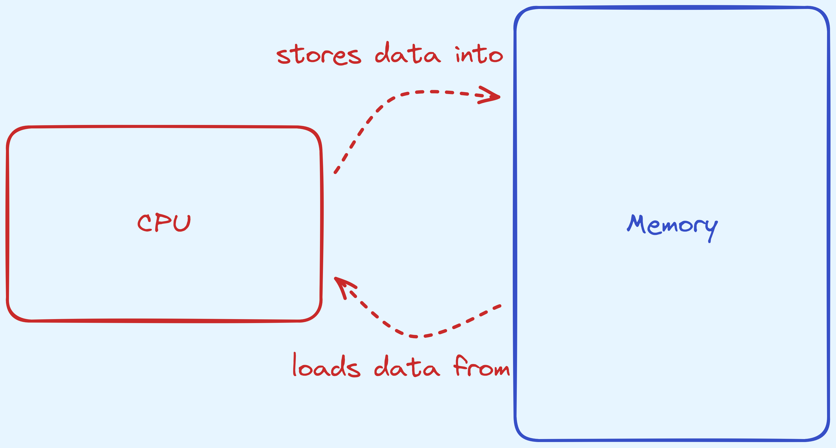
A really simplified model of computation.

We will take it that our memory is randomly accessible. That is to say, that we can access any of the bytes that we want, free of cost. This might be different compared to a model where accessing certain portions of memory might cost differently depending on where in the memory you wish to access, like for hard disks and CDs where we might need to wait for a rotation for locations that are on the other side of the disk.

The CPU, is going to provide an instruction set that we can use. I.e. a predefined list of operations. All of our algorithms that we wish to build, will be using this set, and nothing more. Think of these as the Lego bricks in our playgound.

We’ll first cover what the memory section is like, before talking about the kind of data we will store in them, and then finally the operations that the CPU can perform.

How We’re Using the Memory

In the memory region, we’re going to split it up into two segments. Called the stack and the heap. In reality, your operating system makes both of these segments for each program that runs (along with other segments, but we won’t mention those).

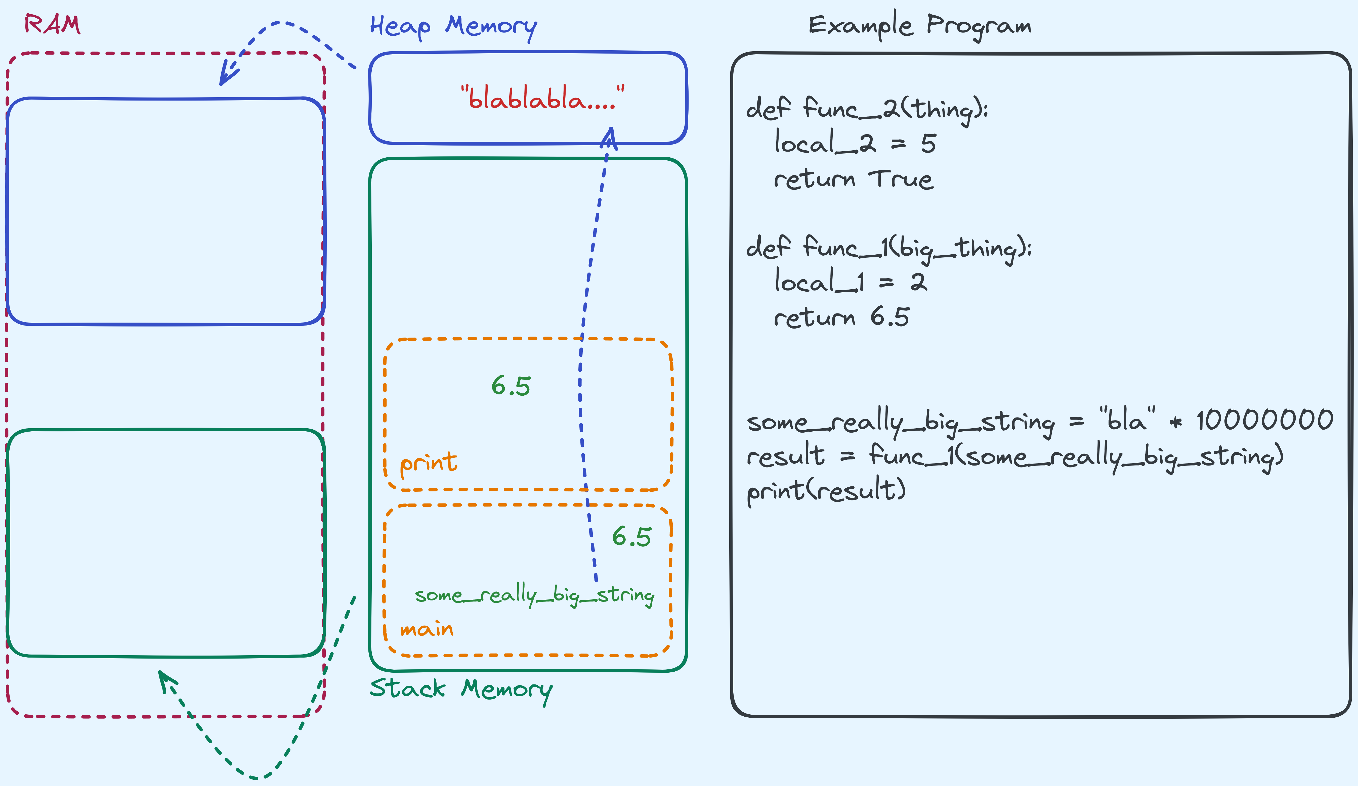
In short, the stack stores data that is local to functions, and the heap stores data that can potentially live as long as the program does.

Here’s an example to show you what I mean:

def func_2(thing):
  local_2 = 5
  return True

def func_1(big_thing):
  local_1 = 2
  return 6.5

# This creates a string that is "bla" repeated 10000000 times
some_really_big_string = "bla" * 10000000
result = func_1(some_really_big_string)
print(result)

For now let’s ignore how some_really_big_string is created. Here’s what the stack and heap look like when func_1 is being called, and when it is calling func_2.

arrays

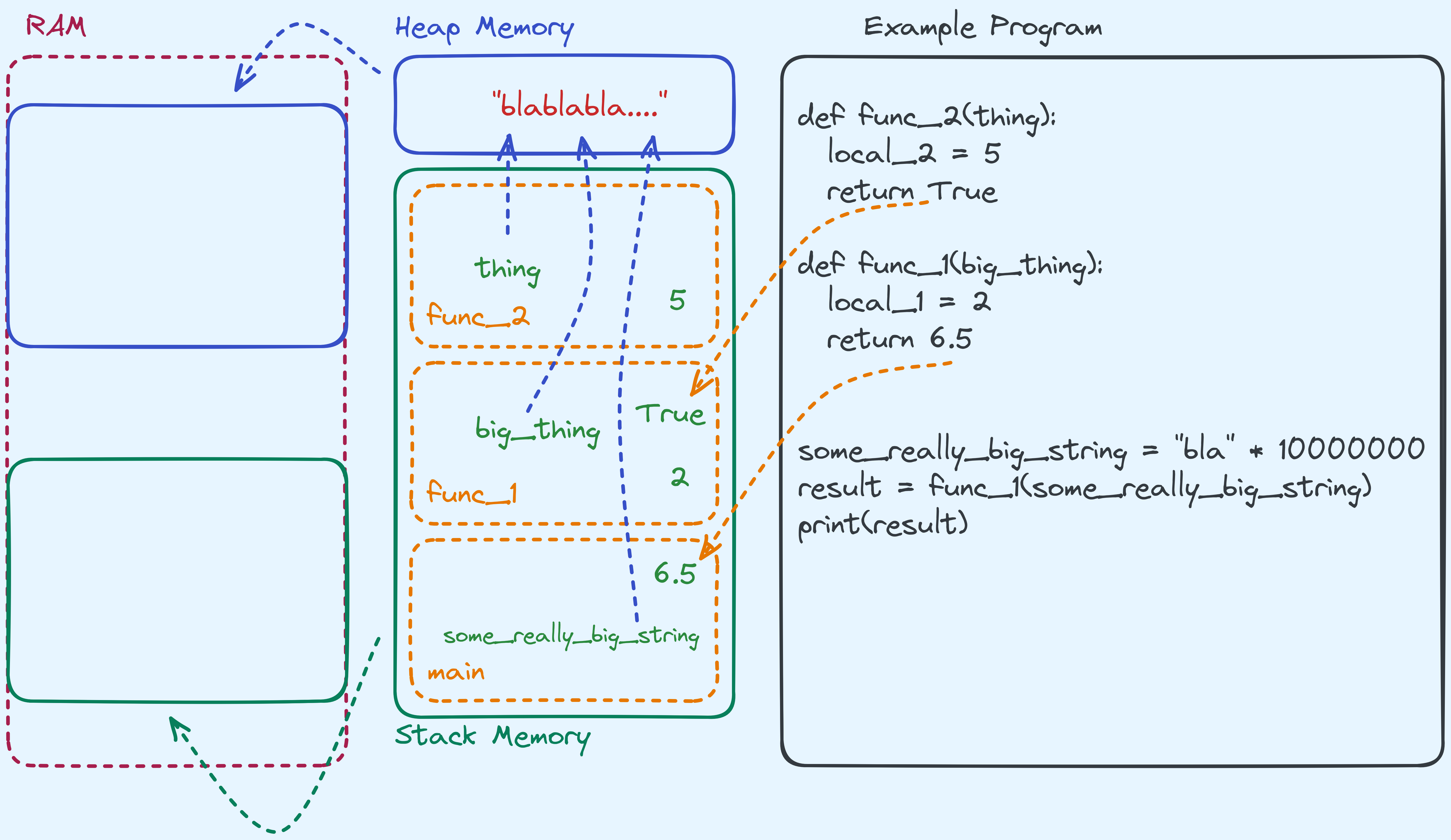
Here are the few things to take note of:

Variables that are local to the function themselves are store on something called stack frames. ² For example, 5 and 2 are stored in their respective frames.
Notice that the string “blablablabla…” isn’t stored on the stack, but the pointer to the string is stored on the stack, and the pointer points to an address in the heap section. At that address, “blablabla…” is written.
The return values are also local variables. If we returned a string, what that actually means is returning a pointer to an address on the heap.

Once the function calls are over, the stack frame is also gone. For example, once we hit the line print(result), the stack segment should look like this instead:

arrays

So as we make different function calls, the stack section grows and shrinks as needed.

So if we contrast these two pieces of code:

  def func_1(a):
    return a + 1
  
  for n in range(10):
    func_1(1)

  def func_2(b):
    if b == 1:
      return b + 1
    
    return func_2(b - 1)

  func_2(10)

An example showing the difference between two functions, both of which are called 10 times.

In terms of how the stack behaves, for the code on the left, expect there to be at most two stack frames at any point in time. Between the calls to func_1, only one stack frame exists. And each time a call to func_1 is done, the stack frame will be “deleted” before the next one is created on the stack. On the other hand, for the code on the right, at some point in time, there will be 11 stack frames on the stack.

In summary:

We’ve talked about the how the memory region is used. We split it into two sections, namely the stack and the heap. The stack grows based on the number of functions being called, and the heap stores longer lasting data, and to refer to it, we pass pointers around. We’ll talk about pointers in slightly more detail later on.

Data Types

The next step is to talk about how we’re going to store data into the memory region — the kind of data that we expect our algorithms to work on. We need to be able to represent (at the minimum) the following:

Truth Values
Integers
Fractions
Alphabetical Characters (and Beyond)
References to Data Objects

The idea is that, these data types are just types of values that we wish to operate on. As we will see, computers need to find a way to store these things, and so we need to represent what we want in a way that the hardware allows for.

Bits

First of all, most modern computer systems ³ like to store information using bits. For our current intents and purposes, you can just take it to mean that anything that we wish to store, the computer has to, and will do it in the form of storing a sequence of values in \(0\)’s and \(1\)’s.

In your RAM sticks, in your hard drives, even when the data is being operated on in the CPU, it’s all really just bits whizzing about circuits.

More commonly, we call every \(8\) bits, a single byte. In fact, we usually index into RAM (random access memory) data by bytes.

Puzzle

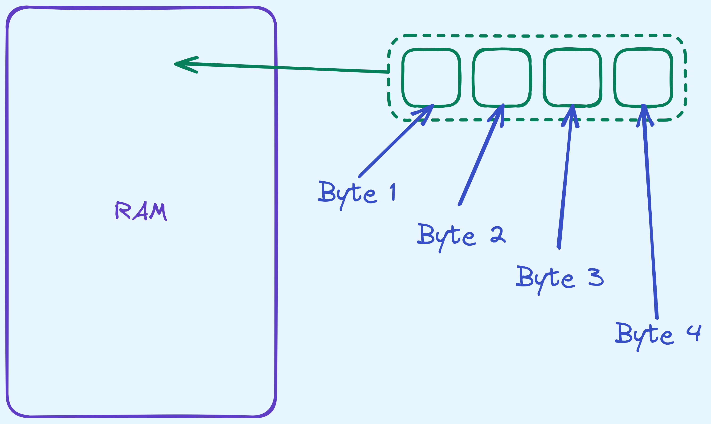
A silly diagram showing what bytes are in RAM.

So for this half of the post, you should take it that when we want to represent certain values, they’re sitting either in RAM, or on a drive as bytes. Let’s see how the most important data types we want are represented.

Booleans/Truth Values

It’s going to be quite common that we need to evaluate the “truth value” of a given statement. Take for example the following that tests to see if a given number a is larger than the square root of another b:

def square_test(a, b):
    # assumes both a and b are positive
    truth_value = (a * a) > b
    return truth_value

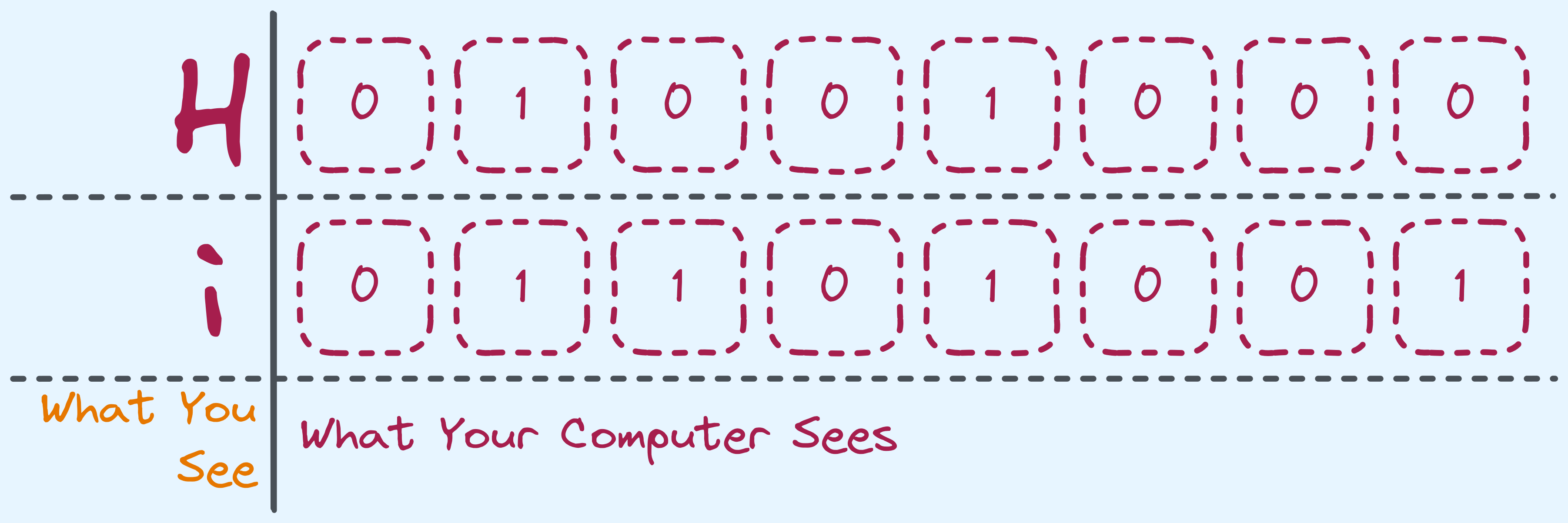
Think for a second about what the computer should store in truth_value if it only sees bits. In Python (or a similar programming language) we expect the type that is returned to be a boolean type that takes on value True or False. Most often, in computers this is represented by 1 and 0 respectively.

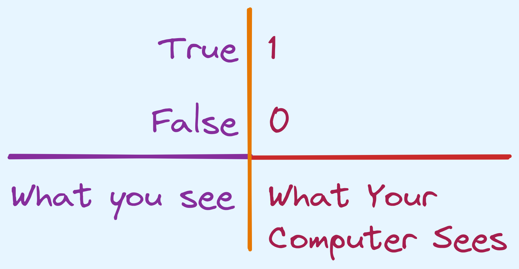How are are representing booleans.

Often times, programming languages also like to treat these as 1 and 0 respectively. For example, in C/C++ it is possible to treat Boolean values as integers and therefore do arithmetic or comparisons with other integers on them. An important distinction has to be made that when a programming language does it, it’s an interpretation that True can be viewed as 1 (and False as 0). Booleans are not integers, after all. They may be represented the same way by computers but semantically, there is a difference between a “truth value” and an “integer”.

Representing Numbers and other Numerical Values

You might be used to seeing integers in represented in base 10, like so:

123
00123
-270

In general, a number in base 10 is represented in the following way:

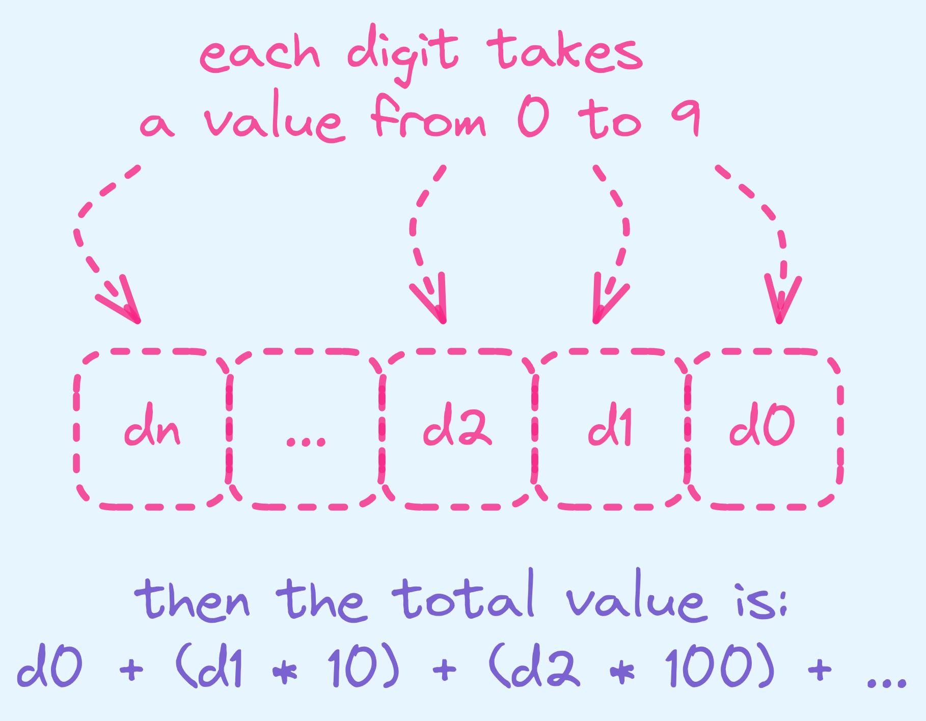Base 10 in general.

However, there’s really nothing stopping us from using base 2 instead. In fact, that’s how your computer stores integers.

Here are some examples:

\[3 = 1 * \left(1\right) + 1 * \left(2\right)\]
\[5 = 1 * \left(1\right) + 0 * \left(2\right) + 1 * \left(4\right)\]
\[13 = 1 * \left(1\right) + 0 * \left(2\right) + 1 * \left(4\right) + 1 * \left(8\right)\]

So in binary, we would represent them like so:

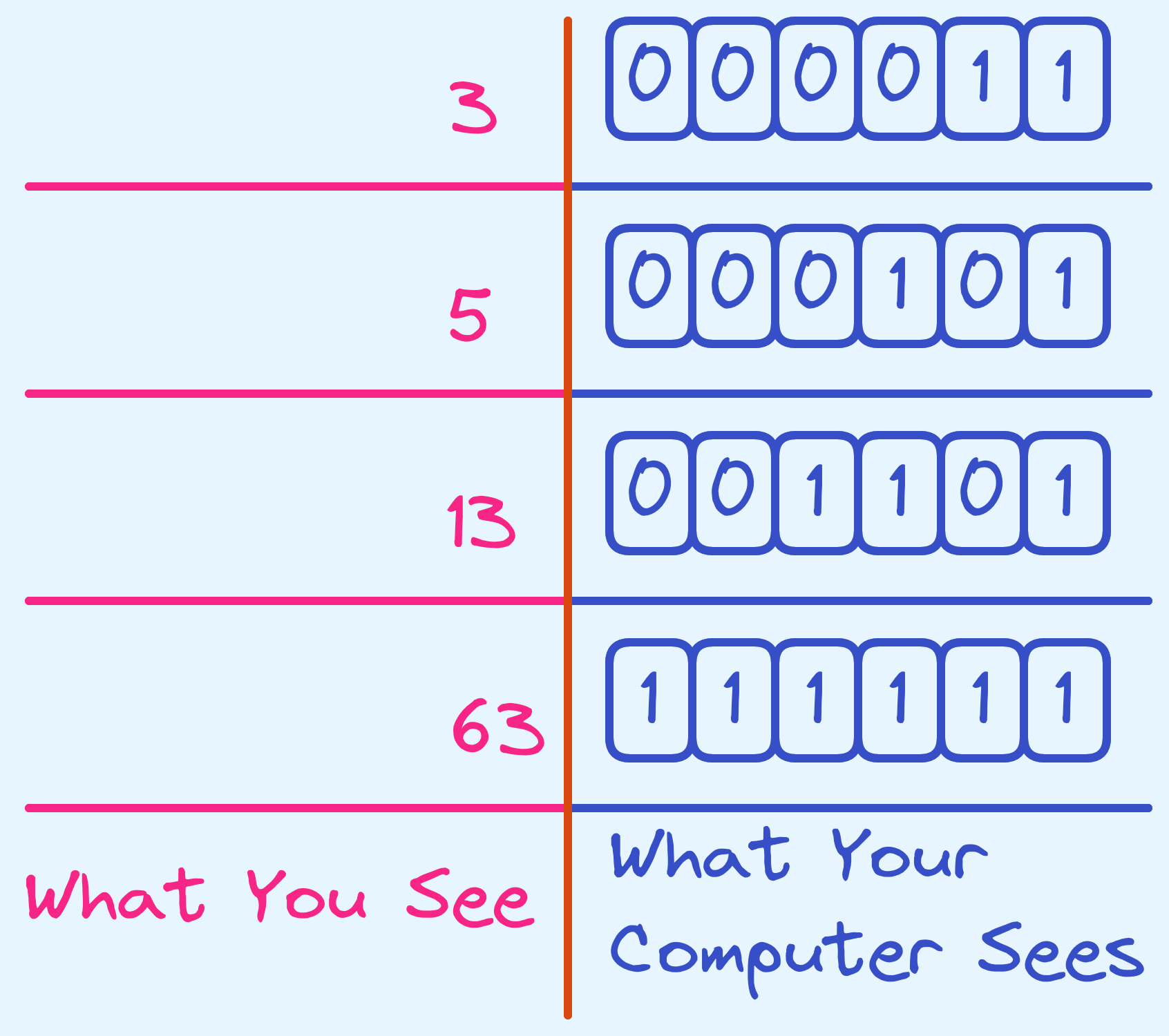example representations What you see as opposed to what your computer sees.

Now theoretically, we could keep this going on forever. A small problem is that the arithmetic logic units (ALU) of modern processors can’t operate on arbitrarily many bits and as a consequence the maximum possible value represented is actually limited. Typically, they allow up to either 32 bits, or 64 bits. So, the largest possible value we can represent up to is either \(2^{32} - 1\) or \(2^{64} - 1\). For convention, whenever concerned, we will from now on take the integer representation to be using \(64\) bits.

Unsigned Integers: For integers that are non-negative, we can store them as unsigned integers in the manner as described above.

Adding Unsigned Integers

Now that we’ve introduced unsigned integers, let’s cover addition up front (because it actually influences the way we represent the other numerical values).

Question: How would you add two numbers in binary?

It’s actually really similar to how you would do it in decimal. Here’s a simple sketch with only \(4\) bits:

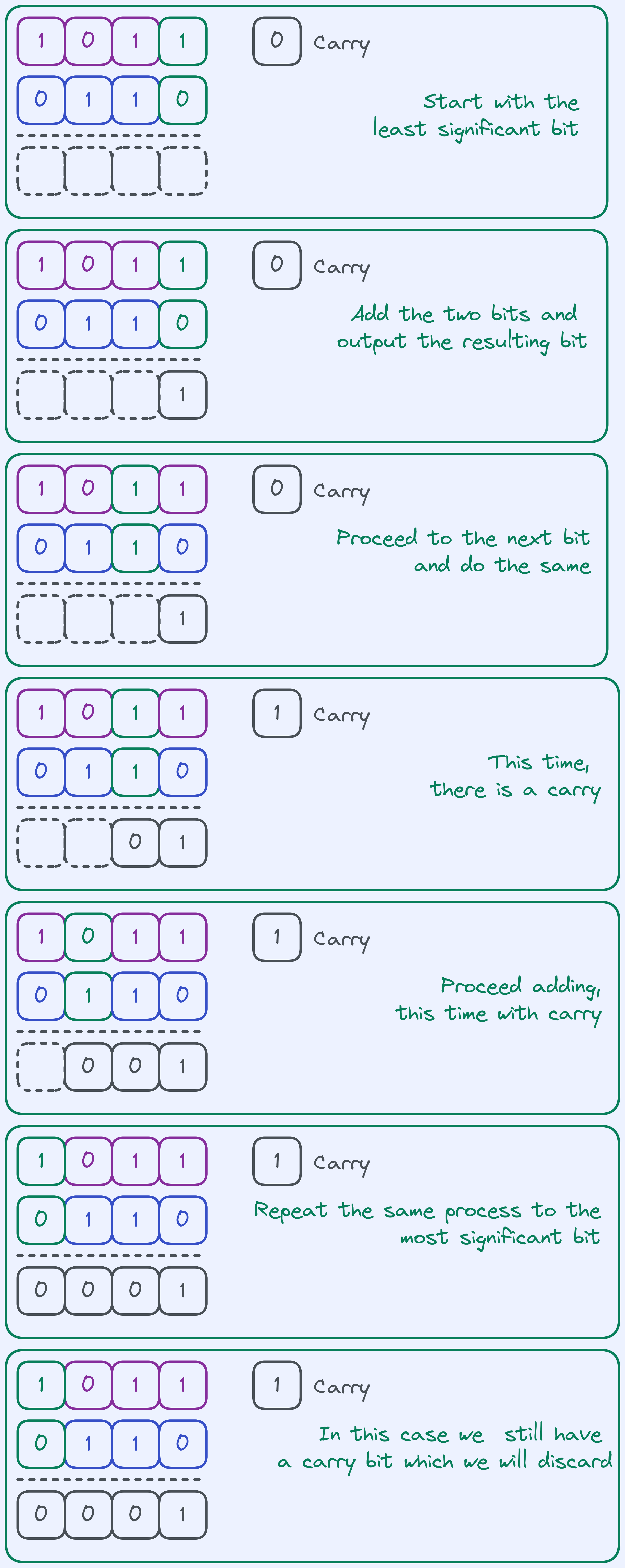Addition algorithm on \(4\) bits.

The fact that we discard the carry at the end makes our addition algorithm behave as sort of a “wraparound”. So really think of this addition algorithm on \(4\) bits as computing \((a + b)\ mod\ 2^{4}\).

Signed Integers

But what about negative values? How should we represent them? One way would be to use one of the bits to mark whether it’s negative.

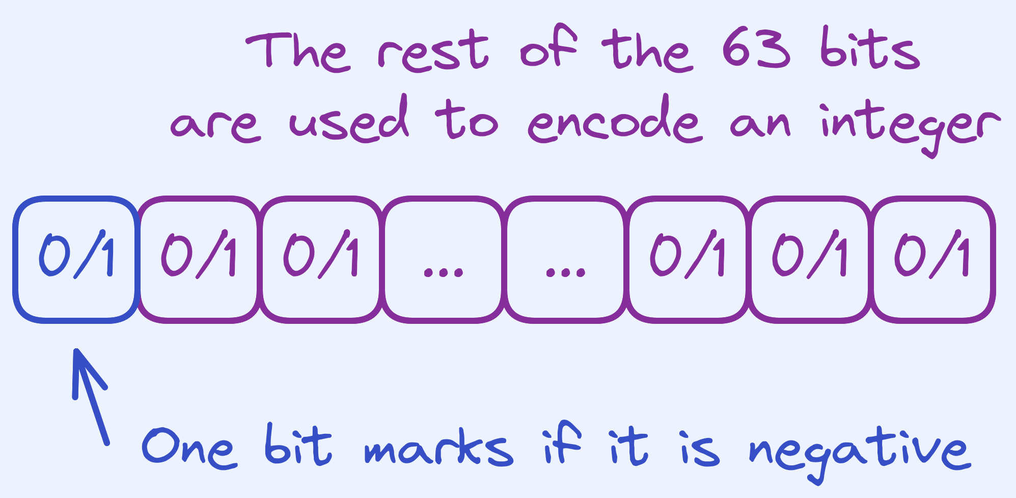Signed Integer Signed Representation.

But then we would need to first check the sign bit to see what kind of integers are involved, and more importantly, based on that we need to either invoke the addition algorithm or a subtraction algorithm.

Instead, it would be ideal to reuse the addition algorithm especially if we can use a representation which doesn’t cost anything (compared to checking a sign bit before invoking either algorithm).

Recall that the addition algorithm we introduced for \(4\) bits basically adds up to \(2^4 - 1= 15\) before wrapping around again. For example, \(2\) and \(15\) would be added to \(1\) (try it). So what we can do, is “reinterpret” the number line from \(0\) to \(15\) to accomodate for negative numbers. You can think of \(15\) as being “\(1\) away from \(0\)” which is basically \(-1\). In general, with \(4\) bits, we would like to think of each number \(-x\) as \(16 - x\). The slight caveat is that with \(4\) bits we can only represent \(16\) numbers, so what we do is spend \(8\) of them representing \(0\) to \(7\), and the remaining numbers representing \(-8\) to \(-1\).

Which numbers we choose to represent.

So if you’re given a number like \(5\) (\(0101\) in binary), what would be its negative equivalent? It would be \(16 - 5 = 11\) (\(1011\) in binary). The nice thing now is that we can add any two numbers between \(-8\) and \(7\) and it just works, as long as we interpret our negative numbers in the way that I’ve mentioned.

Now a “quick” way for computers to convert numbers to their negatives, is to do the following:

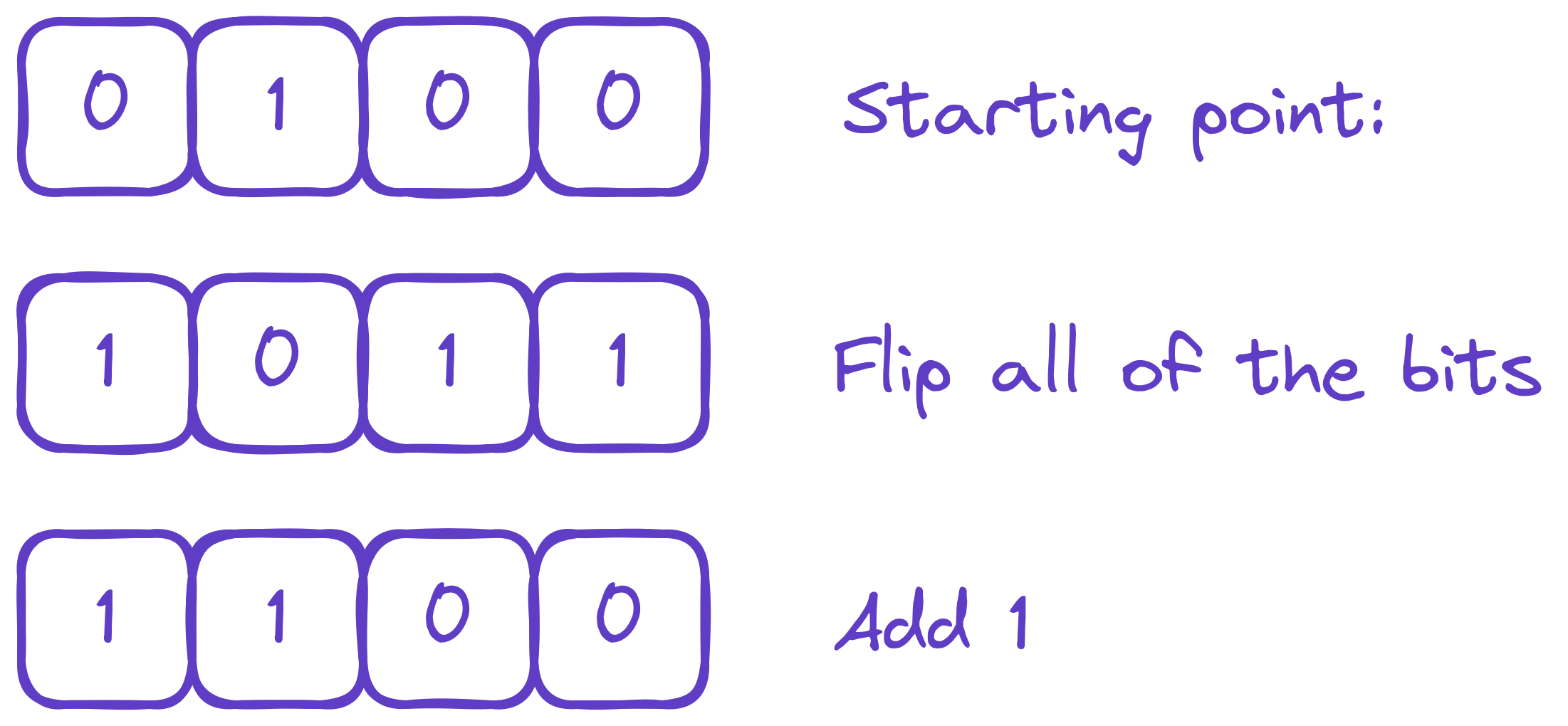How processors actually negate numbers.

This might sound like magic, but that’s really happening is that we’re really just computing \(16 - x\). Think of it this way: \(1111_2\) is \(15 = 2^4 - 1\). So subtracting a number from \(15\) , like \(4\), just removes the bits from \(15\) that \(4\) has. In which case, we would get \(1011_2\). This holds regardless of what number we’re subtracting from \(15\), as long as it’s less than or equal to \(15\) (try it!).

“Removing bits from \(1111_2\)” is really just the same as flipping all of the bits. Now, we really wanted \(16 - x\), not \(16 - 1 - x\). So, what we need to do, is add \(1\) after flipping the bits.

Et voila! Welcome to what is known as two’s complement.

Signed Integers: For integers that might be negative, we can store them as signed integers in the manner as described above.

In practice, you can make signed and unsigned integers for 32 bits, 64 bits, and so on. We can only expect them to go up as large as \(2^{63} - 1\) for unsigned, or \(2^{62} - 1\) for signed integers.

Warning: Note that signed integers and unsigned integers are different types. So adding unsigned integers to signed integers might produce unexpected results since the type tells us how we should be interpreting the numbers.

What about fractional values?

What happens if we want to represent numbers in between integers? What about \(\frac{1}{3}\)? What about \(0.55\)? Relating it back to the decimal system that we’re all comfortable with, we can try a format that looks something like this:

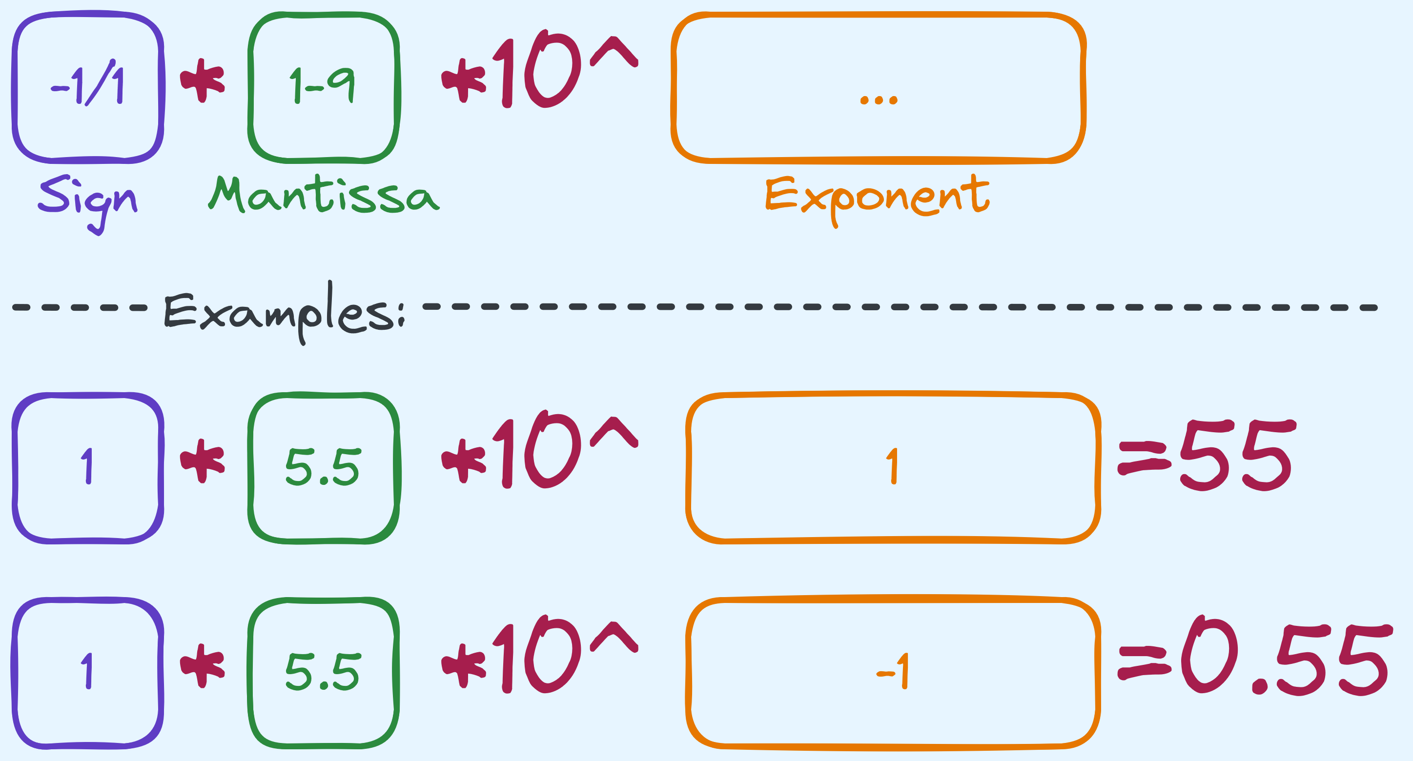An example of how we might begin to start storing fractional values.

We’ve not completely dodged the issue, we somehow still need to store a “fractional” value in the mantissa although now the possible range is restricted from \(1\) to \(10\) (in some sense). Worse still, it’s still unclear how we would store something like \(1/3\), which actually can’t be finitely written in a decimal point system.

The sad fact is that we won’t be able to store values up to an arbitrary precision. As a very simple example, let’s say you only had \(4\) bits for your representation. This means you can only store up to \(2^4 = 16\) possible values. How would you go about storing \(0.3\), \(0.33\), \(0.333\), and so on, up to \(0.3333333333333333\) and \(0.33333333333333333\)? That’s 17 possible values, but with only \(4\) bits, some of these need to have the same bit representation. So instead, the representation that we’re going for, with limited bits means limited precision. Let’s explain what this means in the binary system.

The Fixed-Point System

We’ll start with the fixed-point system.

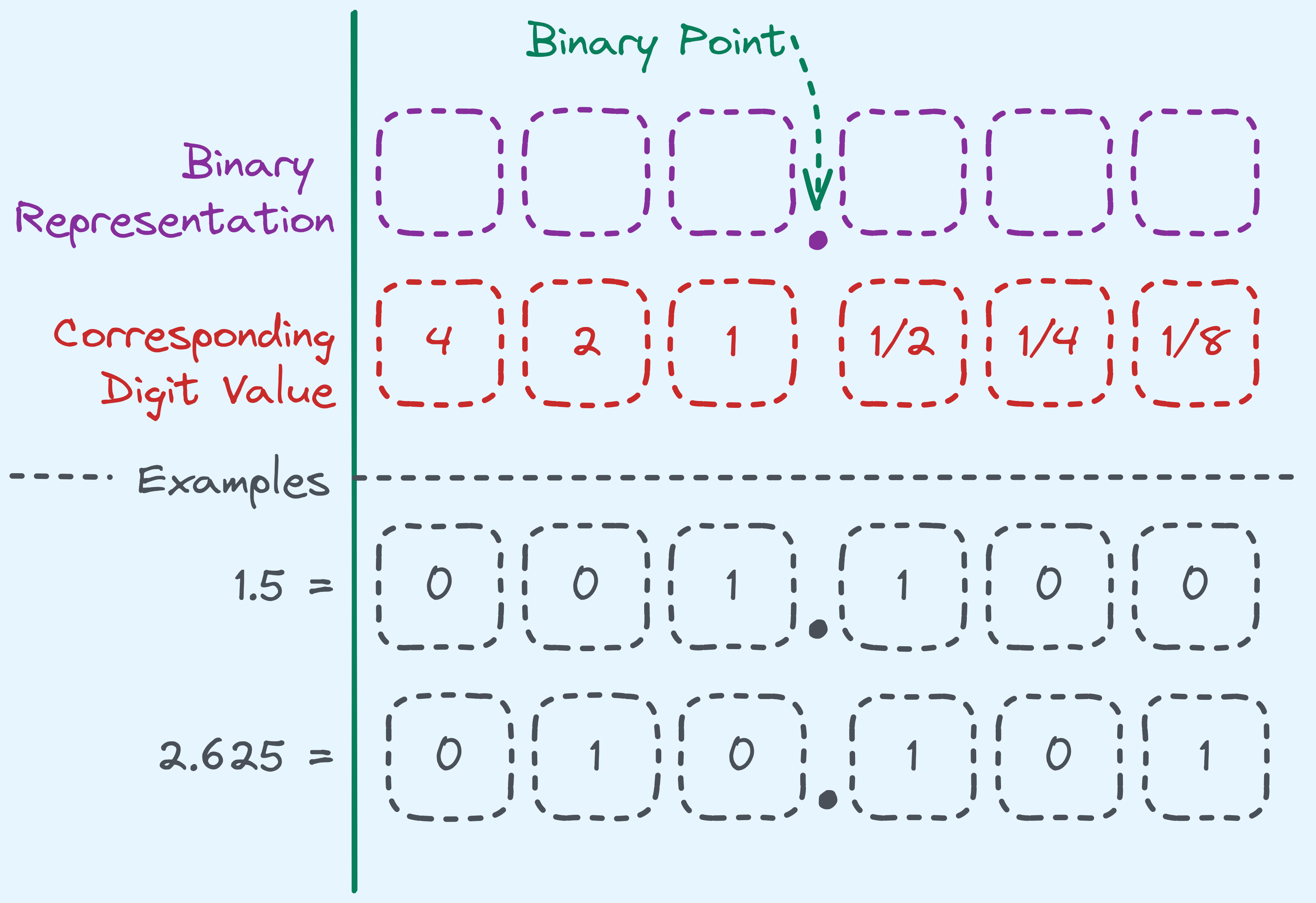Fractional binary values.

The above example is if we had \(6\) bits, and notice that with \(3\) bits for the fractional part, we can store any fractional value in the range of \(0\) to \(0.875\) — basically we have a fixed precision of \(0.125\).

Fixed Point Values: If we want to store fractional values up to a fixed precision, we can store them as a fixed point value in the manner as described above.

The Floating-Point System

But that can be a bit wasteful. We’ve fixed exactly how many digits we can store before and after the point. Consider on the other hand, viewing every value in the following way:

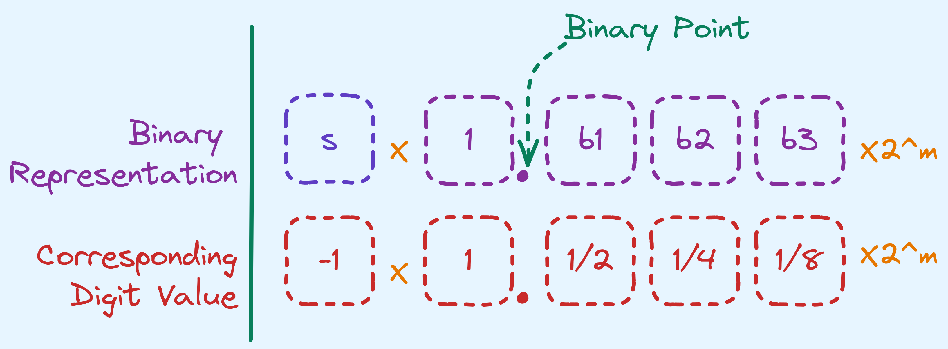Normalised Floating Point Number.

So the rough idea, on how to store fractional values in binary, is the following:

Use 1 bit for the sign.
Use some bits for the mantissa.
Use some bits for the exponent.

So in the diagram above, we’re using \(3\) bits to store a number between \(1.000\) and \(1.875\) in increments of \(0.125\). Some bits are also going to encode an integer \(m\). In practice, when we store \(m\), we start from some negative power, like so: \(2^{-256 + m}\).

Here’s an example with \(8\) bits.

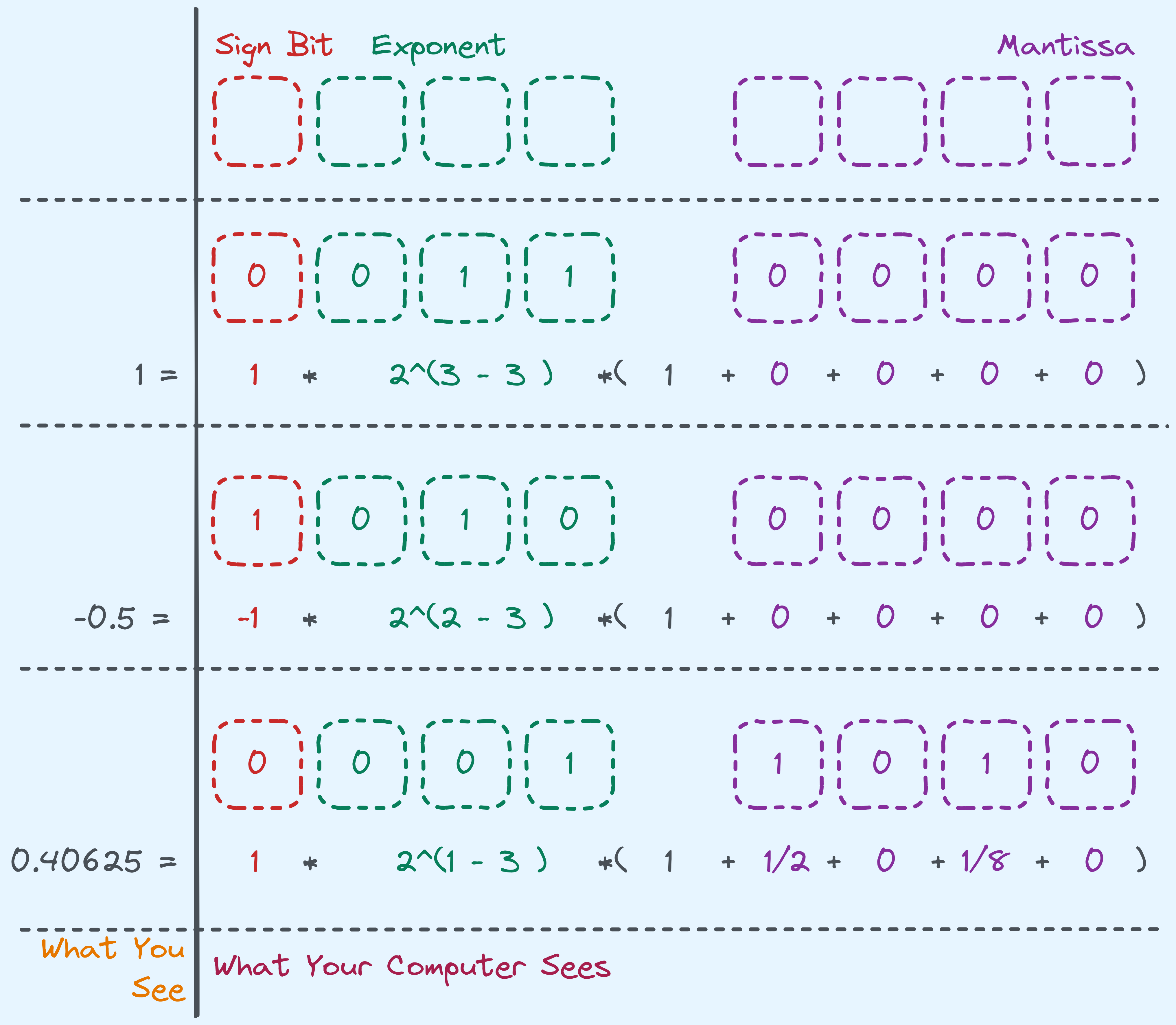Rough idea with \(8\) bits.

The actual way that single and double precision values are represented as specified in the IEEE 754 standard actually has a few optimisations and deals with edge cases that we won’t cover here. Just a simple understanding of how it roughly works is good enough.

For single-precision values (\(32\)-bit representation), \(23\) bits are used for the mantissa, and \(8\) bits are used for the exponent. For double-precision values (\(64\)-bit representation), \(52\) bits are used for the mantissa, and \(11\) bits are used for the exponent.

Floating Point Values: Single-precision binary floating-point values are stored in the binary32 format using 32 bits. Double-precision binary floating-point values are stored in the binary64 format using 64 bits.

Characters

Numerical values aren’t all there is to represent for computers. After all, besides performing mathematical calculations, we might want to manipulate things like databases of names, urls and so on.

The way that this is done is via the character data type. The standard way that characters are encoded is based on American Standard Code for Information Interchange (ASCII).

Here’s a table that maps characters to their values that are stored in computer memory:

ASCII table from www.asciitable.com.

Some notable aspects include that there are non-printable characters in there, like DEL (delete) or NUL (null terminator). Also, besides letters, there are other things that are considered characters, like + or ".

The above table only shows the first \(2^7 = 128\) characters. As a standard, character data types are 1 byte large (or 8 bits), encoding up to 256 characters (the remaining 128 characters are in the extended ASCII table).

How characters are stored.

Nowadays, a popular encoding is the Unicode Transcode Format – 8-bit(UTF-8), which is instead a variable length encoding. It encodes unicode characters, which includes the original set of ASCII characters, and beyond.

Characters: We will can store anything that is ascii encodable as a character.

A Small Puzzle

Here’s a puzzle you can play around with:

Puzzle

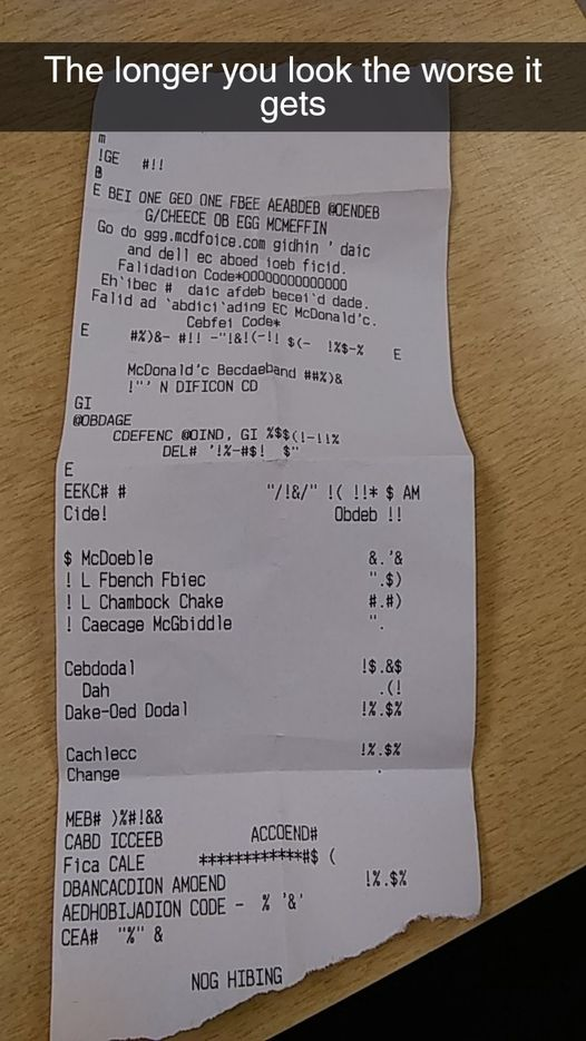
A receipt with some printing errors. Source of image included in solution section.

The original intended text is in English and the hint is that the encoding system used is ASCII. Can you propose a theory for why the receipt has turned out like this? A solution is included at the end of this post.

Arrays, Strings, and Big Integers

It would be handy to store sequences of characters or sequences of other things. An array type can be thought of as a collection of other types. So for example, an array of integers can just be thought of as a list of integers, all stored adjacently. Now this lines up with how hardware stores data.

For our convention of arrays, you should think of them as something that is indexable. That is to say, given an array arr of size \(n\), then arr[0] holds the first element, arr[1] holds the second element, and so on until arr[n - 1] that holds the last element.

For the sake of simplicity, let’s say that we wanted to store 4 integers that are 2 bytes each. This amounts to 8 bytes.

arrays

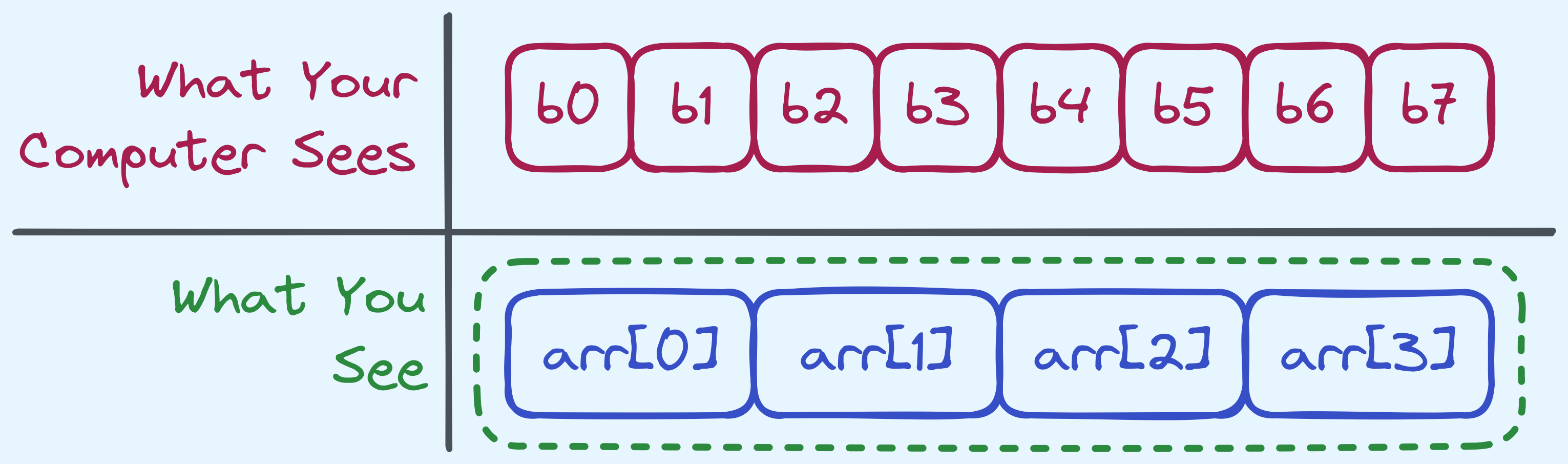
How arrays are seen vs what your computer sees.

Arrays: We will store a sequence of type T as an array of T.

Arrays for common types

So essentially, we can think of strings (sequence of characters) as really an array of characters. The string “Words” can really be thought of as a sequence [‘W’, ‘o’, ‘r’, ‘d’, ‘s’].

Also, recall that the integers we have talked about until now have a limited range of values that they can represent. One thing is that we can represent larger numbers using arrays of unsigned integers instead. Such numbers would have a different base, and each element of the array would represent a digit.

For example, 560 in decimal can be treated as a size 3 array like [5, 6, 0]. There’s nothing restricting us from changing the base of the representation to something else. So if we used an array of unsigned 32 bit integers, we can think of each digit as taking a value in the range of \(0\) to \(2^{32} - 1\) (and thus also the representation as having that base).

In such a case, we would need to implement our own arithmetic algorithms (or rely on a library), since most modern computers don’t support operations for such representations.

Someday I might make a post about big integer representations.

For now, just take it to mean that we can indeed support arbitrarily large numbers if we really wanted to.

How Pointers Are Used

Now the last thing that we need to cover are pointers/references. In programming languages there is somewhat of a difference between what these two objects are, but for the purposes of my series of posts, it will not matter too much.

Let’s first refresh a little bit about stacks and heaps.

arrays

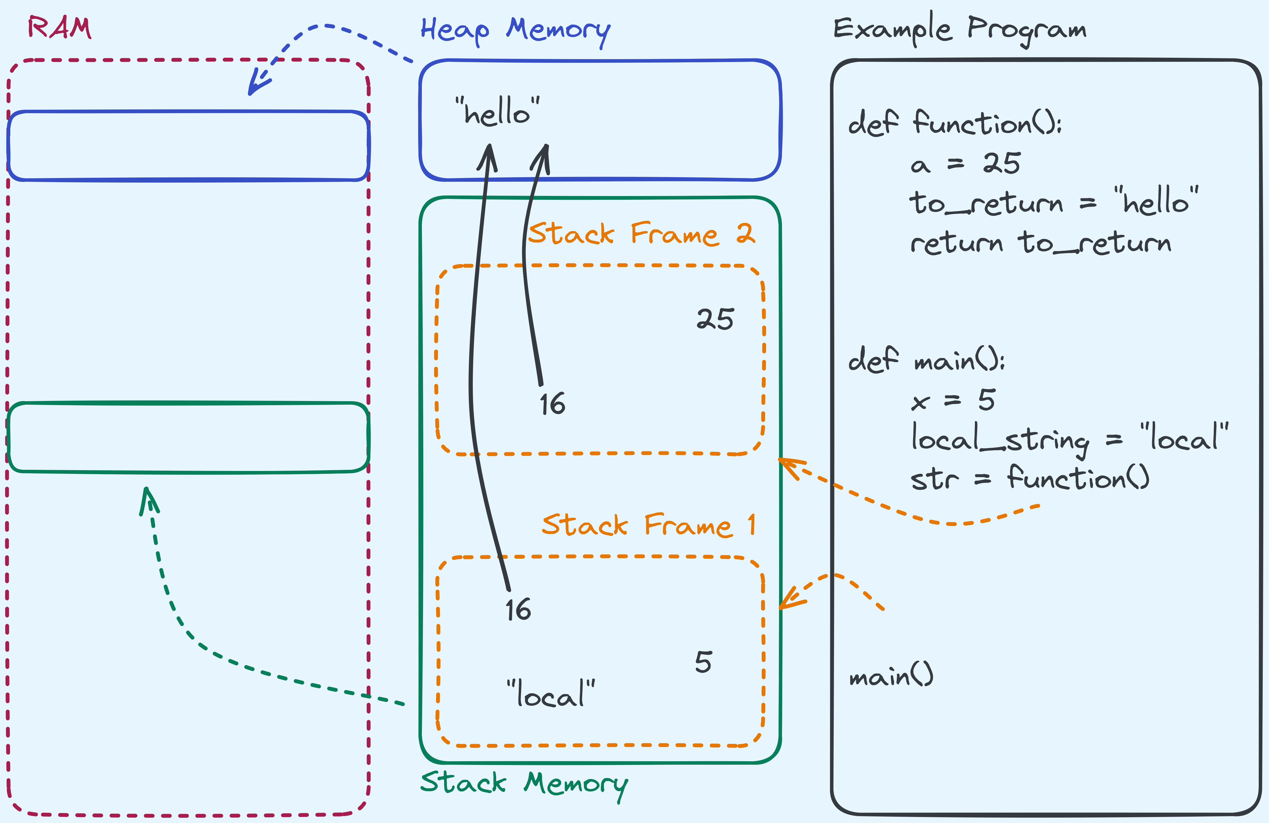
Stacks and Heaps in Memory.

Recall that every time a function is called, a stack frame is allocated on the stack and the local variables (variables local to the function) are stored on the stack frame. In the example above, variables x, a, to_return, local_str, and str are local variables so they are stored on their respective stack frames. You’ll notice that on the stack, values like 25, "local", 5 are present.

But what is this 16? One way to keep something persistent across function calls, is to store it on the heap instead, which is a section that persists across function calls. In fact, data here persists from the start of the program, until the end. For example, "hello" is a string that we would like to keep persistent across function calls, so we should store it on the heap. But how do we let the functions access it? One way is to give it a handle, which is called a pointer or a reference ⁴. When functions are given a pointer/reference, they first need to “dereference” it. What this means is that they need to look at the value itself, in this case 16, and go into the heap and look up memory location 16 (for simplicity, think of this as the 16th byte in the heap) to start getting the string. So a pointer/reference, is not the object itself, but rather an address to where the object is on heap. It literally refers to, or points at, the object we are storing.

Pointers of type T: If a pointer points to something on heap of type T, we call it a T pointer.

So Why Pointers?

This is actually a difficult question to answer right now, but I just wanted to make a section to assure you that most of the reasons will be apparent either later in this post, or a little later on when we talk about data structures.

Composing Into More Complicated Types

Often times, we will find ourselves grouping types together because it will be handle to make our own “types” which are really just composed of the basic types I’ve already mentioned. An example might be a “coordinate” type, which should really just be pair of double precision floating point values.

Another example might be a “person” type, which stores their name as a string, their name as an unsigned integer, and maybe their height, as a double precision floating point value.

One common type that we will talk about later on, is a “linked list node” type, which among other things, stores a pointer that points to a linked list node. We will see what this accomplishes later on.

arrays

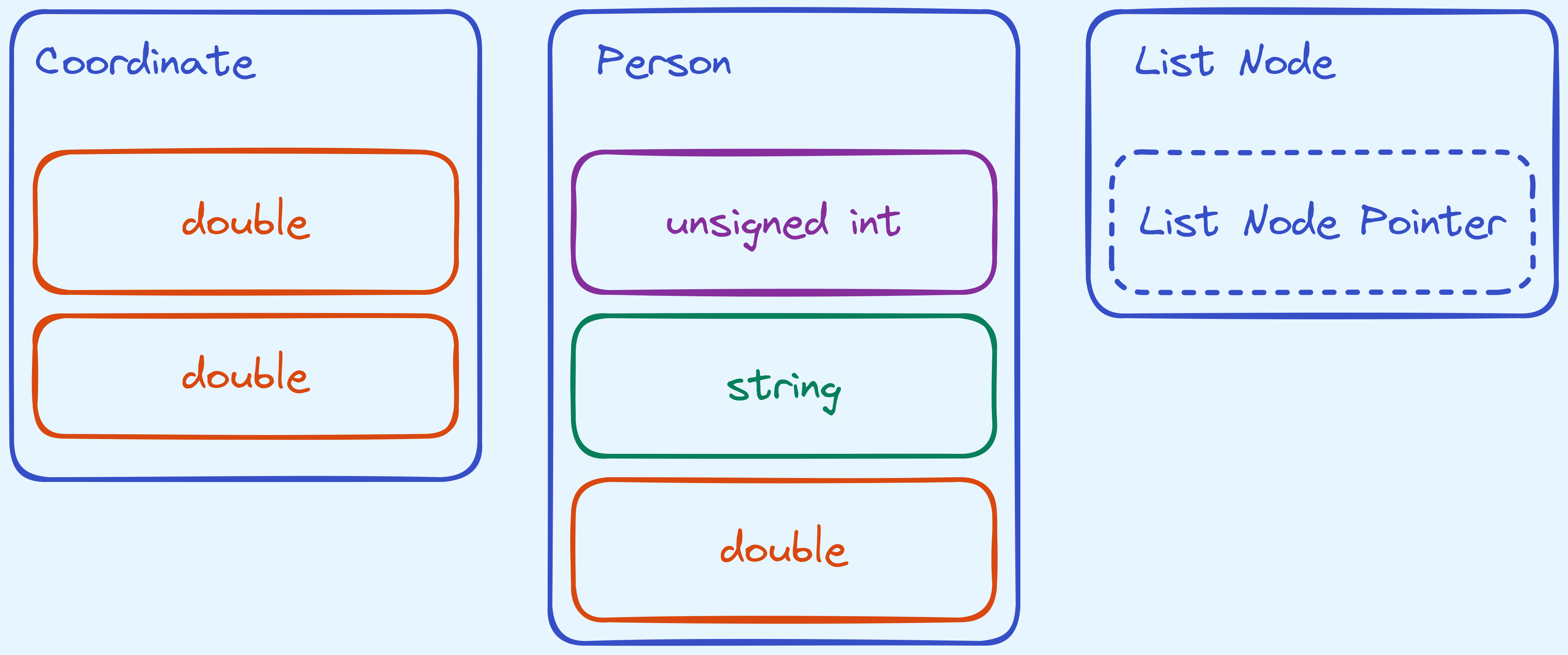
Examples of some composite types we can make.

For now, note that we cannot have a compose a type with itself. Because if we did that, that would be a circular definition! One way around this, is for us to use pointers. I.e. A node won’t hold a node, but rather a reference/pointer to a node.

In Summary:

We’ve covered how we’re going to write and read from the memory regions. And how we’re representing our data.

Basic Operations

Now that we know what kinds of data we can operate on, the next thing to talk about are the kind of operations that we can do on them. Part of the reason this is important is that a big motivation in studying algorithms is trying to count the number of “steps” one needs to take to accomplish any given task. Also, if we don’t specify what are the basic operations that we can make, there’s techinically nothing stopping us from making a “basic operation” that just “solves” the problem.

The Computational Model

We begin by first discussing what should our mental model be for the kind of computation that we can do. We are going to treat our model of computation as really just a CPU and a memory region.

arrays

A really simplified model of computation.

In general, we are going to allow the following operations:

Basic arithmetic (addition, subtraction, multiplication, division, and modulo) for integers and floating point values.
Comparing whether two values are equivalent, or one is smaller than or larger than the other.
Storing single bytes, and loading single bytes.
Testing the truth value of a boolean.
Manipulating bits and booleans with logical operations (AND, OR, NOT, XOR).
Function calling.

Python definitely allows for a lot more operations, we will talk about why we are restricting to a basic set later on. It is safe to say that we are only using Python to express ideas, and our model of computation will depart from what Python does under the hood.

Copying vs. Moving vs. Referencing.

One important thing to note is that we need to at times distinguish between whether we are copying our data, moving it, or referencing it.

arrays

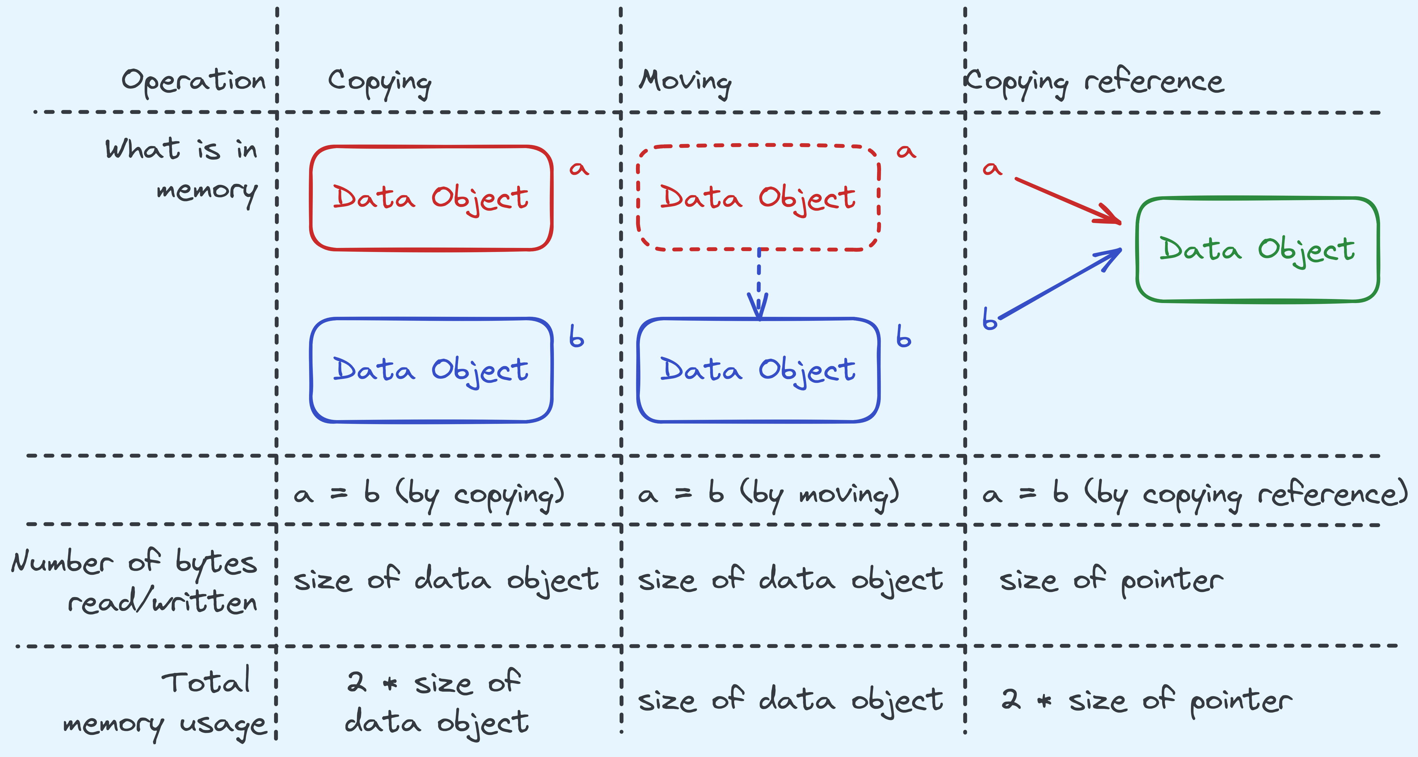
The differences between what we might want to do sometimes.

In certain situations, it will be better to copy objects, but that also means that when we change one copy, the other copy will not be changed. Throughout this series we will be explicit whether we want to copy or move or reference. But in general, expect “small” things like characters, boolean values, integers, and floating point values to just be copied, and “big” things like strings to be referred to.

The Cost of Calling a Function

One very important thing that we will be doing is calling subroutines, or functions. This is a very key operation in algorithm design since we often times want to delegate non-trivial tasks to other algorithms that we can just invoke as a subroutine. Most interestingly, often times we will design algorithms that will invoke themselves again as part of themselves. This sounds circular, but can actually be well defined.

We need to talk about what it costs to invoke a subroutine. When a function is called with some arguments, it generally needs to pass some values in. Furthermore, some space actually needs to be created to hold the values being passed in, as well as accomodate for all the other temporary local variables that it is going to use.

arrays

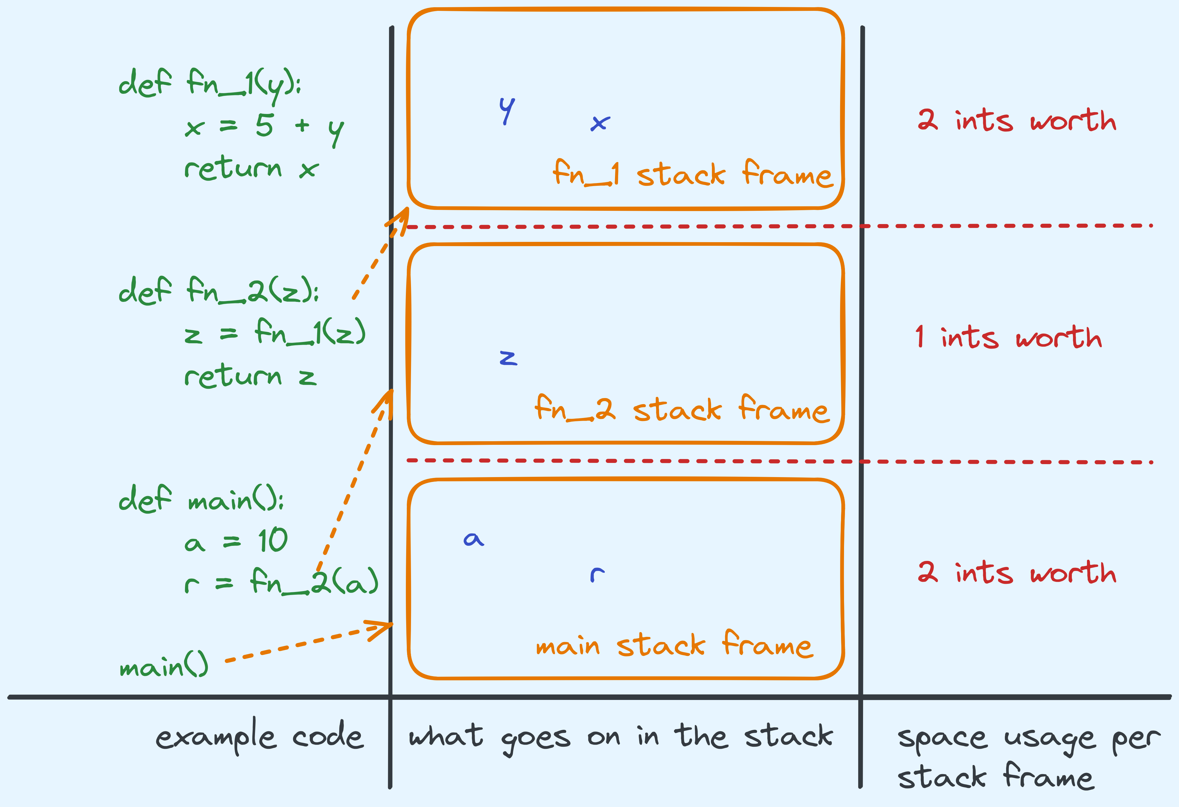
Example of how space is stored.

A Philosophical Aside

Let’s spend a little bit of time thinking about what sort of operations we should really be admitting as single operations. Is multiplication reasonable? What about addition or exponentiation? Some languages like Python offer these like below:

add = a + b
mul = a * b
exp = a ** b

But just because it can be written in a single line or with a single operator, doesn’t actually mean it’s reasonably a single operation. True enough, for things like multiplication and addition, we have circuits for that in most modern processors (among other things). But bear in mind that these circuits accomodate for a fixed number of bits, like 32 or 64 bit values only. What happens if we wanted to operate on much larger numbers? What then?

In an ideal scenario, we want this to model as closely to real life what someone might have to do to computing a value. For example, when you add two numbers with \(d\) digits, how long do you expect that to take? One would take longer to add numbers that are \(10000000\) digits compared to numbers that are just \(2\) digits. So we would expect that the time it takes to compute the addition of two values to be proportional to the number of digits \(d\).

For that reason, in reality we should not expect to be able to even add (let alone multiply or exponentiate) arbitrarily large values in a “single step”. A much more accurate model of reality would be to allow addition and multiplication of values within a certain range. Then, for abitrarily large values, one would expect to represent them as an array of digits, and operations should not be within a single step.

However, for a vast majority of algorithms, the bigger concern isn’t how much these operations cost, but rather how many of these operations that we need to use to get other tasks done. For that reason, it would be a significantly simplifying assumption to accept that these are the basic steps that we can make. But just bear in mind, that in reality, some of these operations should not come “free”.

This goes back to what I said about how models simplify reality enough for us to work with. If we had to worry about every detail that is mostly orthogonal to our actual concern, then we would be very unprodutive in our time in studying algorithms.

In Summary:

We’ve established the basic operations that we can use to build our algorithms. While it is not the most accurate model out there, for the sake of good exposition and learning, it is a reasonable one to work with (in my opinion, at least).

The Efficiency of Algorithms

Alright, we’re mostly done with the low level stuff, and we’re ready to start the covering the basic framework for algorithm analysis.

Time and Space Complexity

As I’ve mentioned, the main concern for the study of algorithms is to make sure that we’re efficient when we go about solving the tasks that we do. This means minimizing the amount of operations that we need to do for solving the same task. More formally, the time complexity of an algorithm is how many operations it takes, with respect to the input size. The space complexity on the other hand, is how much space is used simultaneously at any given point in time.

For example, (and a contrast) here are two algorithms that accomplish the same task of raising a to the power of b.

  def exponentiate(a, b):
      result = 1
      while b > 0:
          result *= a
          b -= 1
      return result

  def exponentiate(a, b):
      
      if b == 0:
        return 1
      elif b == 1:
        return a

      # get the result of a to the power of b/2
      result = exponentiate(a, b // 2)
      
      # square the result
      result *= result

      # if b is odd, we multiply the result by a
      if b % 2 == 1:
        result *= a
      
      return result

Algorithm 1 on the left and algorithm 2 on the right.

What kind of operations are involved in the first algorithm? How many operations do we need? What about the second? Let’s talk about that.

For the first algorithm, it multiplies a to result and subtracts \(1\) from b, \(b\) times before returning the value. We also note that that the initial values of a and b had to be copied in (that’s not a free operation), and one value result was returned (probably by copying to the caller of our function). All in all, that’s about \(2b + 3\) operations ⁵.

What about the other algorithm? This one is a little tricker, let’s first see what it’s trying to do. Basically it uses the following observation:

\[\Large a^b = \begin{cases} \left( (a)^{\lfloor \frac{b}{2} \rfloor} \right)^2 \times a &, \text{if }b \text{ is odd} \\ \left( (a)^{\lfloor \frac{b}{2} \rfloor} \right)^2 &,\text{if }b \text{ is even} \end{cases}\]

See how either way we can do this by calculating \((a)^{\lfloor \frac{b}{2} \rfloor}\)? We can do that by making a function call to exponentiate(a, b // 2) to give us that value. We can then square it and multiply by a again, depending on which case we need. Also, when b is either \(0\) or \(1\), we will immediately return the required value.

Let’s talk about how efficient our algorithm is. At each call of our algorithm makes 3 comparisons, makes one function call (which copies 2 integers), it makes at most 2 multiplications, does 1 modulo operation and returns 1 integer. So that’s about \(3 + 2 + 2 + 1 + 1 = 9\) operations. But wait! When we call the function exponentiate(a, b // 2), this is not a free operation, it actually takes some number of steps to complete as well.

But at least we know that for every function call, it’s about \(9\) basic operations. So the question is, how many function calls do we make at most? Every time we call exponentiate, we divide the value of b by \(2\). So there are \(log_2(b)\) function calls at most. So we need only about \(9\log_2(b)\) operations.

Let’s plot these two out on a graph to see how they compare. (We’ve actually done something similar before in the previous post).

arrays

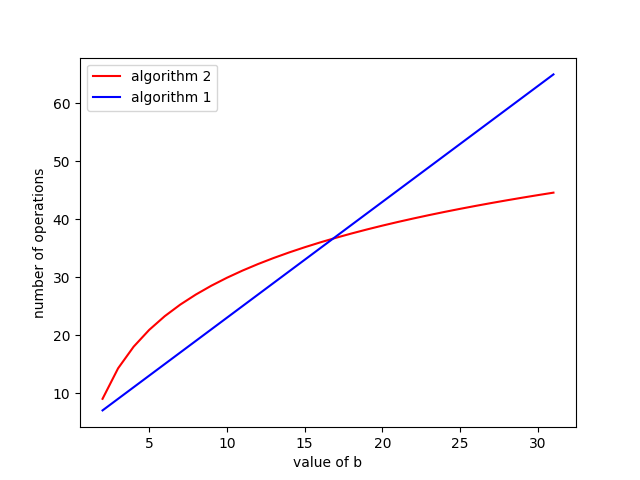
Plot of the number of operations.

From this we can see that when \(b\) is less than \(15\), algorithm 1 costs less, and when \(b\) is a little larger than that, algorithm 2 starts to cost relatively less in terms of time complexity.

What about space? For the first one, we are just storing \(3\) integers throughout the entire computation. So that’s \(3\) integers worth of space used.

On the other hand, the second algorithm actually makes function calls, which, recall actually requires space on the stack. The most amount of space used is when we we call the functions to the point that the last call is either with b being equals to \(0\) or \(1\). There are roughly \(\log_2(b)\) calls before that happens. So the space complexity of the second algorithm is roughly \(3 \log_2(b)\). You could plot a similar graph but in this case it’s a lot less interesting.

The Notion of Asymptotics

This leads into my next point. What should we say about how algorithm 1 compares to algorithm 2? We could say what I did at the end of the previous section but what happens when our algorithms get really complicated and the number of operations starts looking weird?

arrays

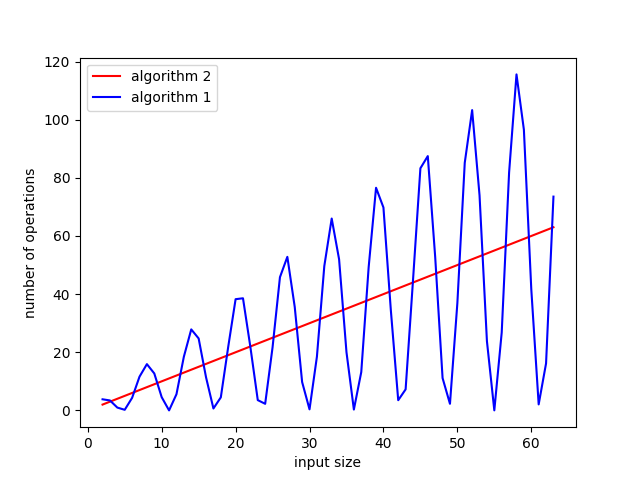
Example of a weird function.

It would be much harder to reason about the relative performance of these two algorithms. Furthermore, one thing we tend to care more about is the general trend of the number of operations as the input size (which we typically call \(n\)) gets larger. So what this is called is the “asymptotic behaviour” of the function.

Note that this is not asking for what the function \(f(n)\) value tends to as \(n \to \infty\), but rather, what is the order of growth of the function (how quickly it grows).

A little informally for now, we would expect functions like \(1000 \log(n) + 100n\) to grow slower than \(5 n^2 - 2000n\) and we would expect functions like \(10^{1000} n + 10^{1000} n^2\) to grow slower than \(2 n^3\). We would also say, perhaps a little counter-intuitively, that functions like \(1000 n\) and \(2 n - 200\log(n)\) have the same order of growth.

The rough idea is that asymptotically, what really matters is just the “fastest growing” term. You can roughly test for whether a term \(f(n)\) “outgrows” another term \(g(n)\) or if they’re on the same order, by evaluating the limit of the following fraction:

\[\large \lim_{n \to \infty} \frac{f(n)}{g(n)} = \begin{cases} \infty &\text{, }f(n)\text{ dominates}\\ 0 &\text{, }g(n)\text{ dominates}\\ \text{otherwise} &\text{, both are on the same order} \end{cases}\]

The point of this is to simplify the otherwise very complicated analysis of how an algorithm behaves. Generally we expect that efficient algorithms tend to perform better as the inputs get larger. That is to say, that at some point, efficient algorithms scale better.

Bachmann–Landau Big O Notation

We are in place to introduce some terminology that we will be using: Big O notation. Formally, we say that \(f(n) = O(g(n))\) if there exists a positive constant \(c\), for all large enough \(n\), it is the case that \(f(n) \leq c \cdot g(n)\). It’s important that you pick the constant first, and same constant holds for all large enough \(n\), rather than having a different constant for every \(n\).

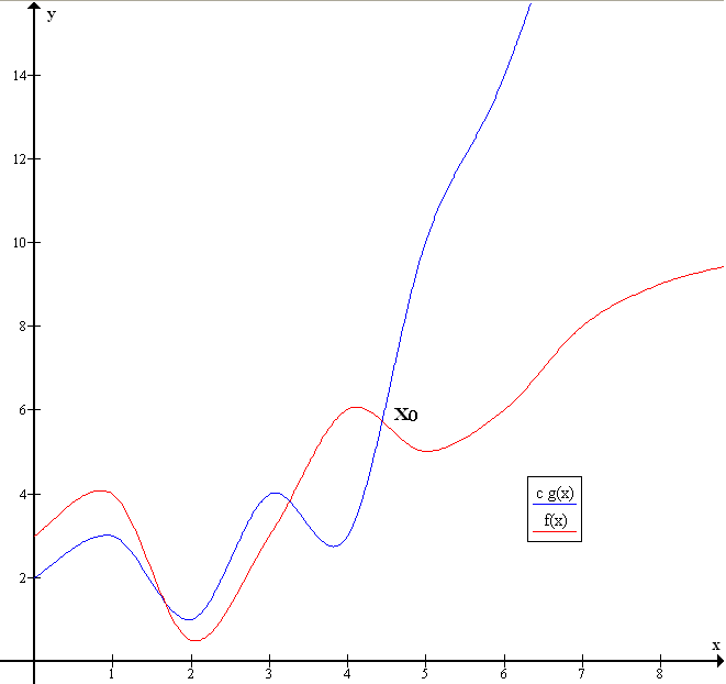
Example of Big O notation. Taken from wikimedia

So based on the example above, we can say that \(f(x) = O(g(x))\) because we can scale \(g(x)\) and find a “starting” point so that from that point onwards, \(c g(x)\) is always greater than or equals to \(f(x)\).

So for example, \(5n^2 - 200n = O(n^2)\), \(500 = O(1)\), and \(9\log_2(n) = O(\log(n))\). Bear in mind that big O only cares if you’re “less than or equals to”, so it is not wrong to say that \(n^2 = O(n^3)\), but it is definitely incorrect to say that \(n^3 = O(1000 n^2)\).

Relating back to our previous example, we would say that algorithm 1 has a time complexity of \(O(b)\) and a space complexity of \(O(1)\). On the other hand, algorithm 2 has a time complexity of \(O(\log(b))\) and a space complexity of \(O(\log(b))\).

There are other notations that will be useful eventually, but we will talk about them in the advanced section of this series.

In Summary:

We’ve talked about the most common objective in basic algorithm study — asymptotic efficiency. In the next post we will start covering algorithms under this framework.

Where the Real World Departs From The Model

There are merits and of course, downsides to the model I’ve introduced. Let’s cover the downsides now so we at least know what to bear in mind for the rest of this series.

The Limits of Asymptotics

As I’ve mentioned, when considering the asymptotic time/space complexity of an algorithm, we’re expecting that for sufficiently large inputs, the order of growth to be small. Whatever the input size before our algorithm kicks in, is not a concern. This leads to algorithms that are seemingly efficient but actually impractical for actual use. Algorithms that take this concept to the extreme are known as galactic algorithms.

The other thing is that we ignore constant factors in the complexity of our algorithms. What this means is that, for example two algorithms might have have time complexity \(O(n)\) when the underlying constant factor vastly differs and we would accept both as being similar or otherwise the same.

Key Takeaway: Just because something is asymptotically efficient, it does not make it a good algorithm for practical use. Some algorithms allow for better implementations, whereas others provide good theoretical guarantees.

The Cost Of Accessing Memory

Under our model, we are assuming that memory accesses anywhere cost the same amount of time. In reality, modern CPUs employ memory caches. When data is loaded, an entire line of bytes is read from memory into a small memory unit called the “cache” which is physically placed much closer to the CPU.

What this means is that accessing adjacent memory locations actually costs vastly differing units of time. In practice, algorithms that make use of this fact often run faster and are favoured over algorithms that do not.

Key Takeaway: Not all memory accesses are created equal. Subsequent accesses to adjacent memory locations are typically faster than to locations that are spread out.

The Cost Of the Different Operations

Besides memory accesses, operations actually have different costs as well. Floating point arithmetic operations have a significant cost compared to integer arithmetic operations, for example.

In fact, depending on the certain architecture we’re working on, the actual costs very significantly. GPUs might have better ALUs for floating point arithmetic than CPUs, for example.

Key Takeaway: Not all operations are created equal. Depending on the architecture and underlying circuit design, the costs of operations vary significantly.

All the Other Complicating Factors

Nowadays, besides what I’ve mentioned, there’s other things like vectorisation, prefetching for both memory accesses and instruction accesses, branch prediction, and so on. All these factors actually make a significant difference in how fast your programs run, and make the difference between what sort of algorithm you should choose to implement. An algorithm that allows for these optimisations to kick in albeit being asymptotically sub-optimal, might actually be much better in practice, than algorithms that don’t but are asymptotically optimal.

Granted, these optimisations I’ve mentioned only introduce constant factor improvements, but in a real world setting, these typically end up winning out on realistic inputs.

That said, there are recent studies in algorithms that model these improvements and try to formally make use of them. We will talk about this at a much later juncture.

Key Takeaway: What we model for algorithms is not the end of the story. Theoretically good algorithms are far from perfect, and for real world use, a lot more thought has to be put into what is considered good.

How about we run benchmarks? Can we use that to justify what we want?

Well it really depends on what you want. Do you want to assess how your implementation runs on a specific input set? Can you guarantee that your tests are comprehensive enough to cover all the cases that your algorithm needs to deal with? Would the conclusion of your tests be applicable to other machines?

There are also “issues” with benchmarking instrumentation. Depending on what you use, it might not be an accurate reflection of what the algorithm is really doing. Some are less intrusive and use a sampling method with hardware interrupts. Some are a lot more intrusive and keep a very close eye on all the resources being used. Either way, some form of observation affects the overall experiment itself. While it is true that there exist really good tools out there that do their best to measure and at the same time minimise their footprint, you have to bear in mind that there are limits to what the experimental approach can do.

Also, on actual systems, it’s quite typical that other processes need to be running in the background. Perhaps your algorithm might be preempted throughout its execution and that might cause issues like cache thrashing, for example. Having to account for all these external factors is difficult.

Is that the sign of a bad algorithm? Hardly.

Should we still take a theoretical approach?

Is there a point to algorithms that are only theoretically efficient and aren’t practical?

Depends on who you ask.

For people who wish to understand this facet of applied mathematics, and people who enjoy the abstract ideas of computation, absolutely. I think the study of algorithms from this theoretical perspective has a lot to offer and new dimensions of thinking that are quite fun, and at the minimum (at times) useful in random daily life tasks.

For anyone who has a more practical use case in mind, I would still argue that the ideas here are important as a foundation. One should build up their toolbox and the whole point of taking a simplified view at first is so that one can get used to the basic ideas before considering them again in a wider setting.

Also, note that sometimes (not always), theoretically efficient algorithms come before practically fast ones.

What Next?

Great! We’re somewhat done with the foundation that we need. Head on over to the next chapter whenever you feel ready and we can start building some algorithms.

Epilogue: Puzzle Answers

Notice that some words remain unaffected, like the word “Change” ⁶. Let’s look at some of the ascii values for the characters in that word.

Character	ASCII Value	Binary Representation of ASCII Value
C	67	01000011
a	97	01100001
n	110	01101110

See how the 5th least significant bit is always 0, and furthermore for any of the other bits, they they seem to be unaffected. (We can’t test the most and second most sigificant bit using this word).

The leading theory could be that the 5th least significant bit is stuck on 0, whereas all of the other bits are kept faithfully. Let’s test this out.

Let’s use a word like “McDoeble”. You can check that the ascii value every character in that word does not have the 5th bit in its binary representation. The original word should be “McDouble”, and lo and behold, the ASCII Value of ‘u’ is 117, or 01110101 in binary. If we mask out the 5th bit, we get 01100101 in binary, 101 in decimal, or the letter ‘e’!

Equivalently, “Fbench Fbiec” should be “French Fries” and if you check the relationship between ‘b’ and ‘r’ or the relationship between ‘c’ and ‘s’, you’ll notice that indeed the 5th bit is always set to 0.

So in all likelihood, the 5th bit is stuck somehow. How might that be? Receipt printers are usually connected to cash registers via ribbon cables, like the one below.

Puzzle

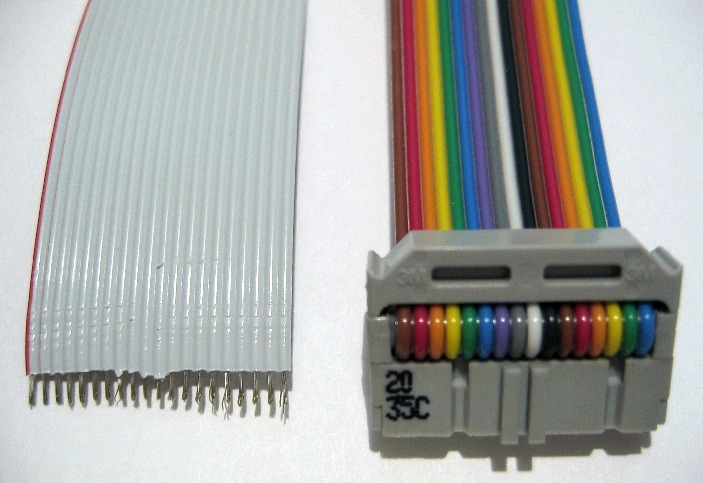
An image of two ribbon cables, taken from Wikipedia.

That’s multiple parallel wires that supply information to the printer. One guess is that there were 8 of such parallel wires that would send out 8 bits for the letter encoded in ascii, and the 5th wire was frayed or the connection was loose, so the bit was always stuck on 0.

Now this isn’t an isolated incident. In computer RAM, sometimes bits can be stuck too, and when your computer reads the bits from it to print characters, the same thing happens.

Stuck RAM Bit

Stuck RAM Bit Causing Print Issues, taken from Imgur.

Hope this was fun!

the stack instead, but we’re going to simplify things.

Things like out of order execution on the CPU, how the OS that it’s running on might allocate memory, what the behaviour of the underlying language (and version of that language) that it gets interpreted into. ↩
In practice, stack frames store a little more information but let’s just leave it as this. ↩
I say most, because things like ternary CMOS and quantum computers exist. ↩
It is common in programming languages that there are subtle differences between what the terms “references” and “pointers” refer to, but let’s not go into that. ↩
The more astute of you at this point might realise I’m not actually very rigorously counting the number of operations, we’ll get to that in a minute. ↩
Which is ironic because it remain unchanged during printing. Haw haw haw. ↩