A First Look

Prologue

Alright! Let’s begin our foray into algorithms. The first concept we’re going to cover is recursion. This is going to be a key tool in algorithmic problem solving. In my experience at least, often times (but not always) problems can be first viewed this way for a potential solution. So, it will be the very first thing to add into our toolbox.

Recursion

Recursion in our context is when an algorithm invokes itself, often (but not always) on a “smaller” input. The idea here is that sometimes, problems are really just made up of identical but smaller problems.

To be a little more precise, we can define algorithms based on themselves. While this might seem circular, if we do it properly it all works out.

A few key features of recursive algorithms include:

1. Having something called a base case. This is the smallest case of the problem that does not invoke the algorithm itself again. ¹
2. Breaking down the current problem we’re solving into smaller versions of the same problem. It need not necessarily be so small as to be the base case. But we should eventually get there.
3. Using the solutions to the smaller problem to help solve the bigger problem. Sometimes this step is trivial, sometimes this step is a little more involved.

Post Organisation

In this post we’re going to first show a few problems, and how they can be solved recursively. We’ll just cover the basic idea to introduce you to it. This post will be really light, because we’ll be using it a lot more throughout the entire course so you’ll be getting practice that way.

The intention behind this post is to give you only an introduction to what recursion is, so at least starting the next post, we are already okay with the ideas.

We will also cover some analysis, but nothing too formal, we’ll save that stuff for after building up some experience.

Then after all that, I’ll cover Karatsuba’s algorithm. A really cool algorithm on how to quickly multiply integers.

Typically, most content I’ve seen would first cover a lot of cases for analysis before giving the algorithms themselves. I’ve decided to do this a little differently becase I think it flows better that way. And, because we’re not constrained by the time frame of a single semester.

And then in the second half of this post, it’s bonus content that is optional, but I think provides some really nice background on stuff that happens in practice, for recursion.

---

Recursion, The Idea

Let’s run through the idea of recursion first. We won’t be too formal, I just want you to get used to what it is sort of like first. Then, after we know a little more, we can delve further into it.

Binary Search

Binary search! We’ve already seen this previously but let’s cover it formally. As I’ve mentioned, binary search is a very common algorithm and is a very handy tool that is often times used as a building block for other things. The problem to solve is as follows:

Binary Search:

Input: You are given an array of \(n\) values as arr. The values come in non-decreasing order. You’re also given a value as query.

Problem: Decide if query exists in arr.

Let’s do an example where we’re given arr is an array of \(n\) integers.

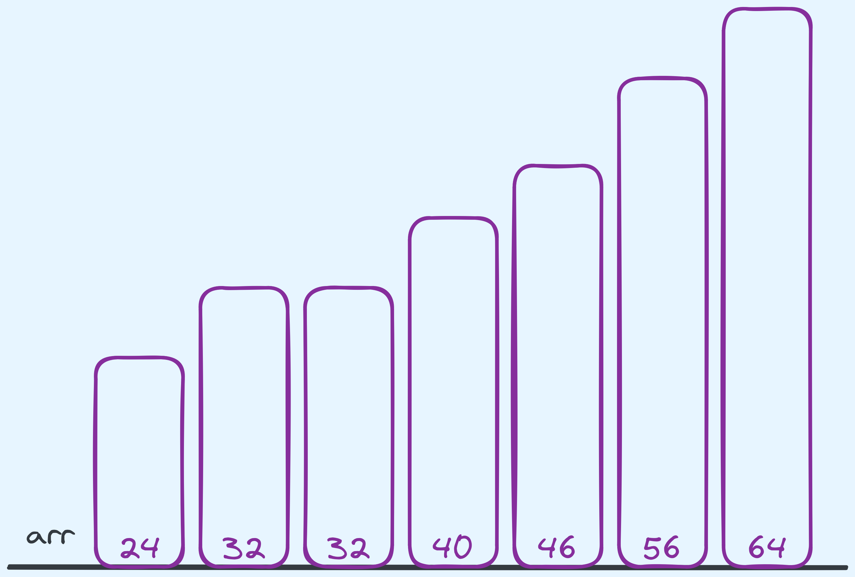
Example input for binary search.

Let’s say that we were searching for \(46\). Now the idea is to start in the middle of arr, and we compare against the the value found in the middle. Now \(46\) is larger than \(40\), so based on that comparison, we know that if \(46\) is to be found, it has to be in the remaining portion of the array that is to the “right” of the middle.

So at this point, we recurse on the right half of the array, by choosing to binary search on the remaining part. That’s it! In our algorithm we do nothing else. The subsequent problem will be solved by a separate instance of binary search.

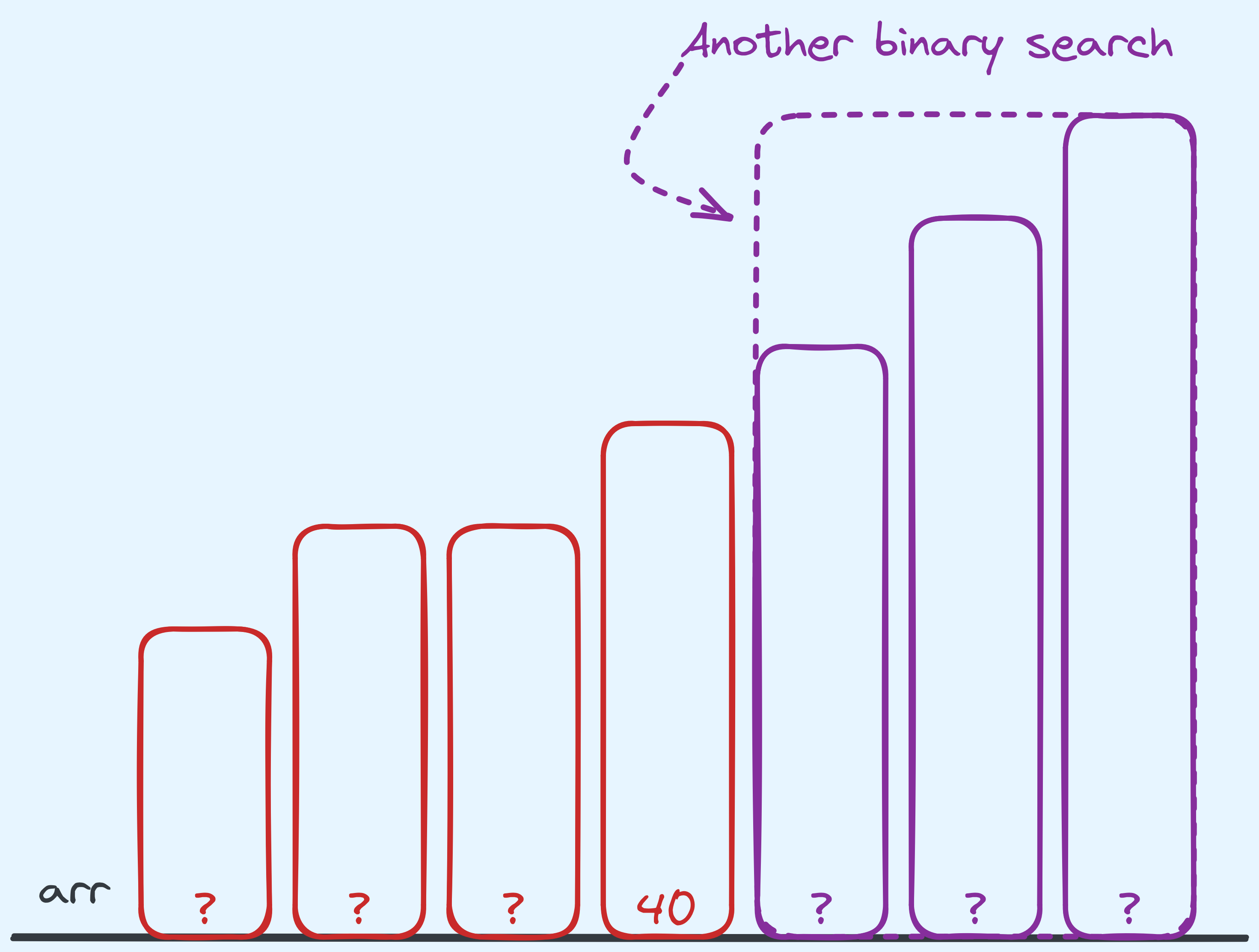
What one instance of binary search deals with, and what it doesn’t.

Notice how our algorithm does some work, then decides how to “break” the problem into a smaller one. In our context, we make the observation that searching for \(46\) basically boils down to searching for \(46\) in the right half of the array. Wahey! It’s the same problem but on a smaller portion of the array. So that’s how we’ve decided how to decompose the problem.

In some sense, in one step of binary search, we only really “see” the middle value, and the rest of the values are not of our concern. Once we’ve seen it, we can decide which half of the array to invoke a new instance of binary search on, and that instance does its own thing and if we trust that it works and gives us the correct answer, we can forward their answer to the question of whether query exists.

The last thing we need to concern ourselves with is a base case. I.e. the smallest version of the problem we do not recurse on. A safe one would be an empty array. That’s the smallest possible case that we don’t have to recurse on. When the array is empty, we know that we didn’t find the value we were looking for, so we return False.

Now of course what happens in reality (for this example), is that the algorithm does something along the lines of:

1. Start in the middle, sees \(40\), recurses on the right side.
2. Start in the middle of the right side, sees \(56\), recurses on the left of the right side.
3. Start in the middle of the left of right side, sees \(46\), realises we have found the value.
4. Returns True.

If we were searching for something like the value \(1\) instead, the algorithm does this:

1. Start in the middle, sees \(40\), recurses on the left side.
2. Start in the middle of the right side, sees \(32\), recurses on the left of the left side.
3. Start in the middle of the left of left side, sees \(24\), recurses on the left of the left side.
4. Realises that there’s nothing left of the array, returns False.

So, in Python, the code might look like this:

def binary_search(arr, left_bound, right_bound, query):
  if left_bound > right_bound:
    return False
  
  middle_index = (left_bound + right_bound) // 2
  if arr[middle_index] == query:
    return True
  if query < arr[middle_index]:
    return binary_search(arr, left_bound, middle_index - 1, query)
  if query > arr[middle_index]:
    return binary_search(arr, middle_index + 1, right_bound, query)

An example implementation of binary search.

This implementation has a few points that we can discuss, but for now as an idea, this is about it.

Factorial

Let’s consider another problem that I think very naturally has a nice recursive structure.

Factorial:

Input: Given positive integer \(n\) as an input.

Problem: Output \(n!\).

In case you don’t know, \(n\) factorial (denoted by \(n!\)) is usually defined in the following way:

\[n! = \begin{cases} n \times (n - 1)! &, \text{ if }n \geq 1\\ 1 &,\text{otherwise} \end{cases}\]

The definition itself is already recursive. The base case is when \(n\) is \(0\) and otherwise, we compute the \((n-1)^{th}\) factorial and multiply it by \(n\).

def factorial(n):
  if n == 0:
    return 1
  
  return n * factorial(n - 1)

An example implementation of factorial.

Again, notice how in the algorithm we deal with the base case (when \(n\) is \(0\)) and otherwise we delegate the job of computing the \((n-1)^{th}\) factorial to another call of our own algorithm.

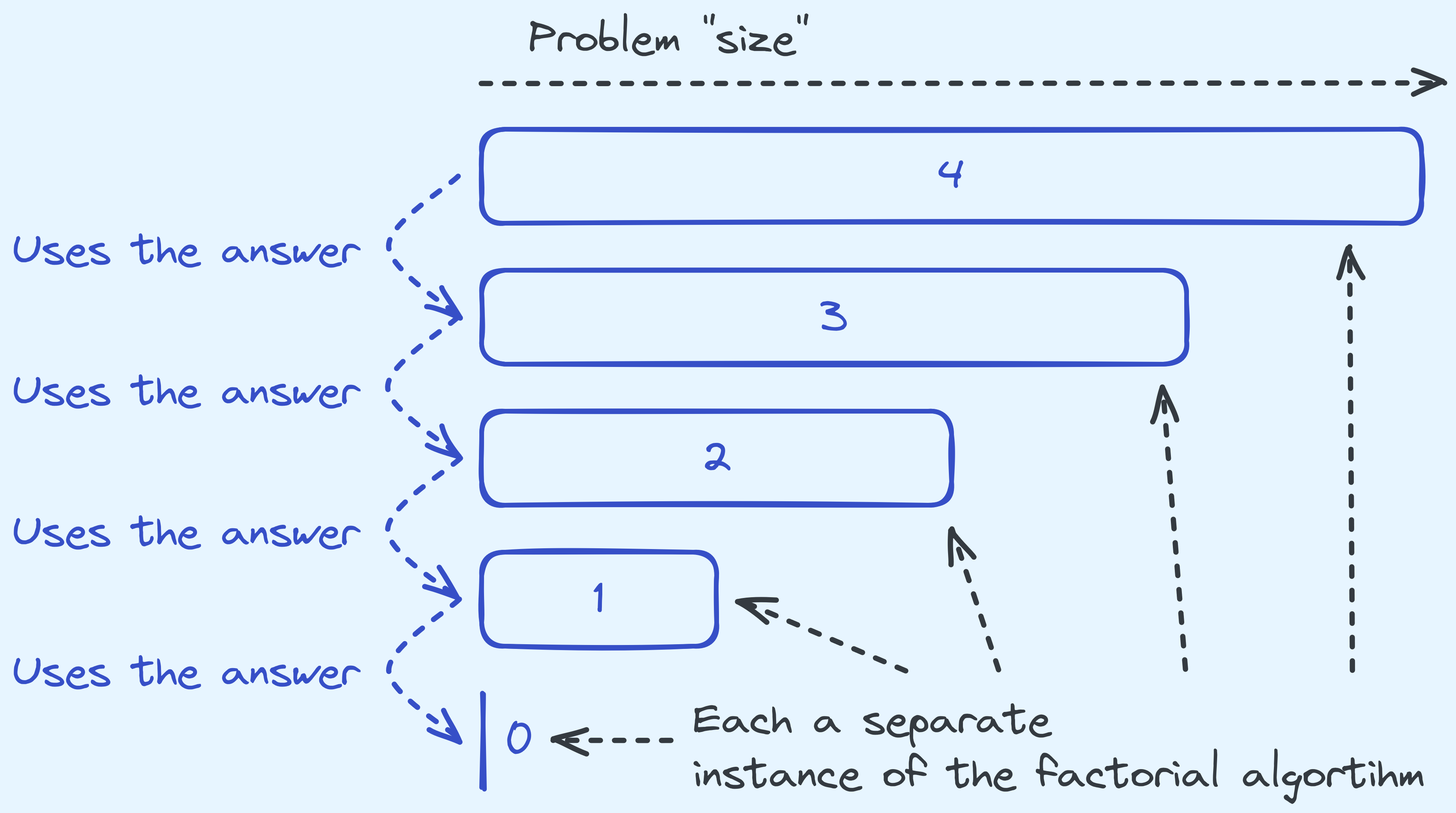
How the instances of the factorial algorithm relate to each other.

Unlike in the case of binary search, here we’re recursing on problem instances that are only “one smaller”.

Also, more notably, in the binary search case we can happily forward the result along. But in the case of this algorithm, we need to take the value, and then operate on it before returning the final value.

Climbing Stairs

We’ve talked about problems that only make a single call to itself, let’s look at something that makes two calls. There’s nothing stopping us from making multiple recursive calls.

Stair Climbing:

Input: Given positive integer \(n\) as an input. You start with at the first step of the stair. You can either:

1. Take the next step.
2. Skip the next step and take the one after that.

Problem: Output the total possible ways you get get to the \(n^{th}\) step.

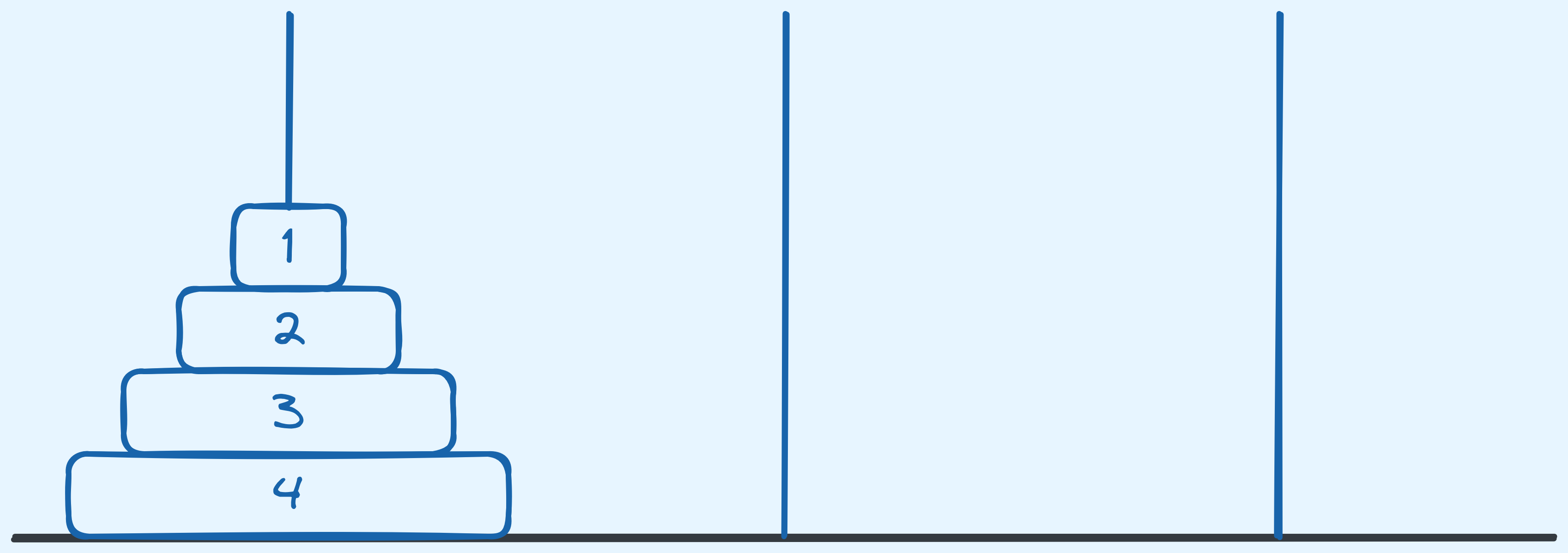
So for example, if \(n\) is \(4\), here are the following possible ways:

Possible ways for 4 steps.

So how do we solve this recursively? Let’s think about it. Let’s say that we had already taken a step. Then we are left with \(n - 1\) steps, which we can traverse in any way we wish to the \(n^{th}\) step. We could also take \(2\) steps now, and then we are left with \(n - 2\) steps instead. So the total ways for \(n\) steps, is the total ways with \(n-1\) steps plus the total ways with \(n-2\) steps.

The two possible cases to recurse into.

So let’s identify some of the base cases. If \(n\) is \(1\), then we know that there is exactly \(1\) way for us to reach the \(n^{th}\) step: Just do nothing. If \(n\) is \(0\), there aren’t stairs in the first place, so there’s \(0\) ways. (Think about what happens when we “overshoot” the stairs. Then there are \(0\) steps of stairs left.)

What about the recursive cases? We need the solution to \(n-1\) and \(n-2\). Then we add them up before returning the value.

def stairs(n):
  if n == 0:
    return 0
  if n == 1:
    return 1
  
  return stairs(n - 1) + stairs(n - 2)

An example implementation of stair climbing.

Exercise: Tower of Hanoi

Alright! Let’s give as an exercise, the following classic problem whose solution is motivates recursion.

Tower of Hanoi:

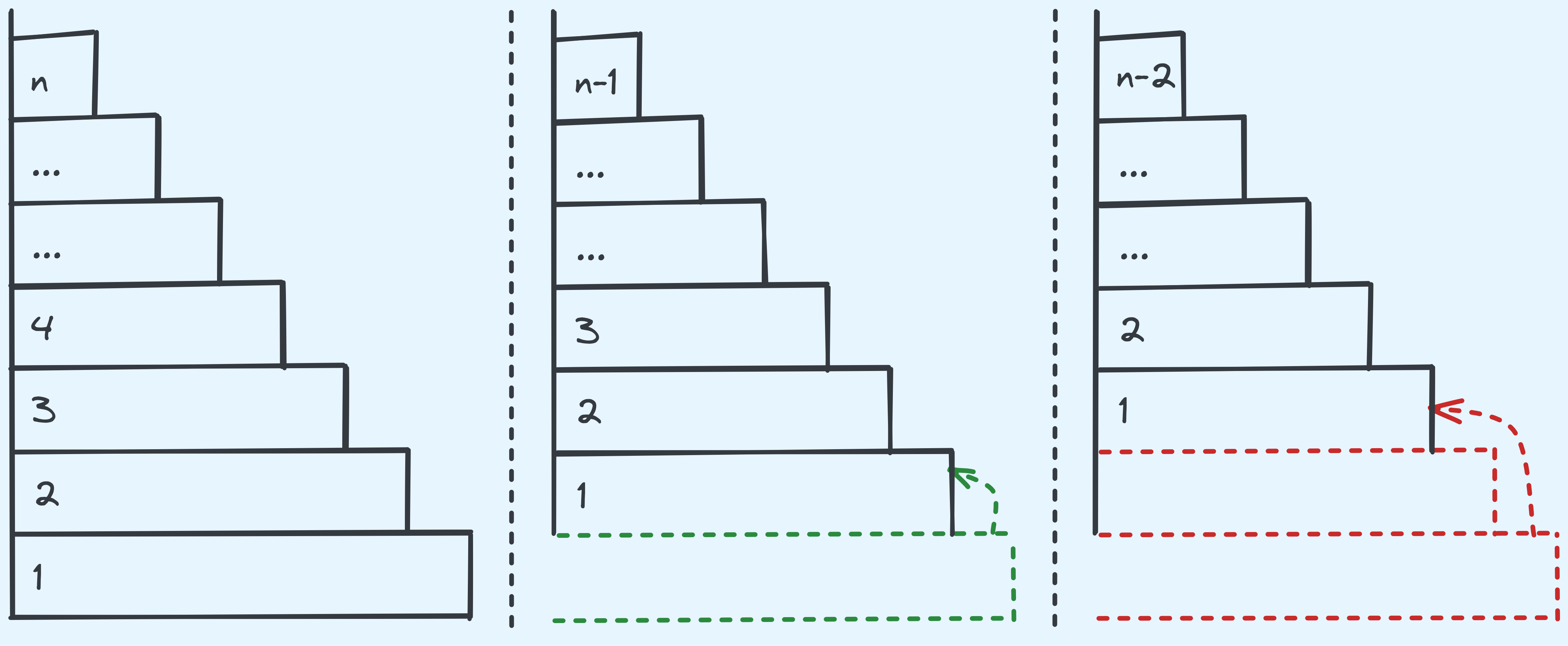
Input: You’re given \(n\) stacks of disks. The lowest disk has width \(n\). Each disk stacked on top is \(1\) less in width. The smallest disk has width \(1\).

Here are the rules:

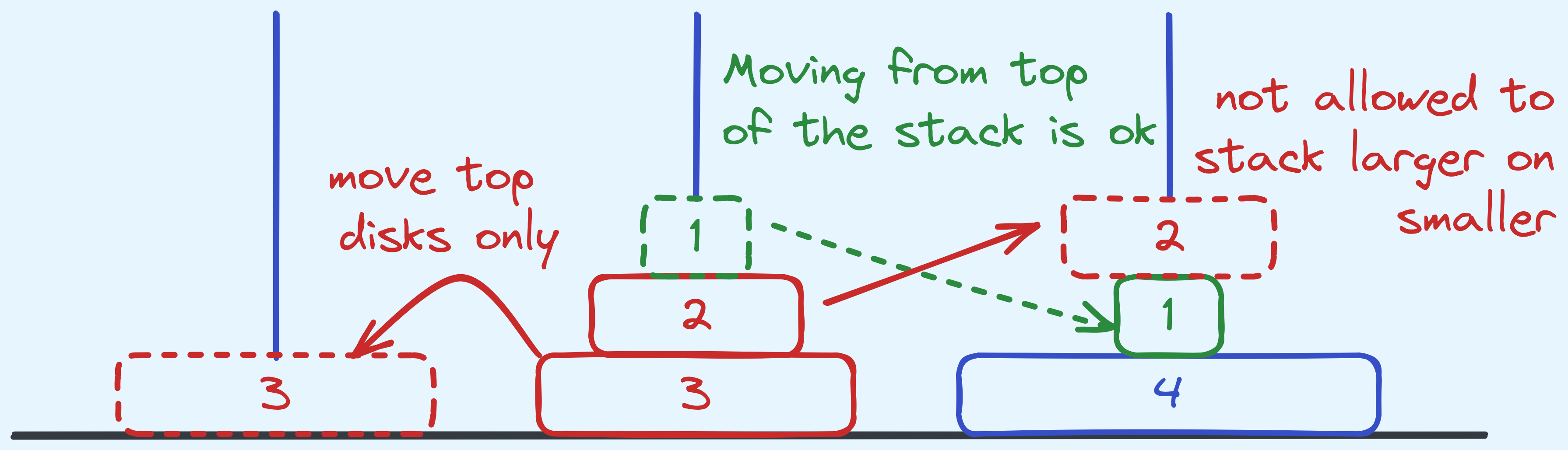
1. There are three possible stacks. The first has all \(n\) disks arranged as mentioned. The next two are empty.
2. You may move only one disk at a time between stacks.
3. You can only move the disk that is at the top of a stack.
4. At no point should there be a wider disk stacked on top of a narrower disk. If a stack is empty, you can move any disk to it.

Problem: Given \(n\), output the sequence of steps that moves all the disks from stack \(1\) to stack \(3\). A step can be given in the following form: “Move from top of stack x to stack y”. Since we can only move the top disk of the stack at any given point in time, there is no need to mention what the width of the disk is.

The solution will be covered at the end of this post. Happy solving!

Recursive Problem Solving in General

Alright let’s talk about this a little more formally.

Recall a little while ago, we mentioned that recursive algorithms tend to have a base case. And otherwise, they break problems into smaller versions of the same problem, obtain a solution and sometimes operate on top of that before returning an answer.

Formally, this is called decomposition into smaller sub-problems, potentially, recombination into a solution. This is more commonly referred to as “divide and conquer”.

Throughout this course there are going to be many algorithms that are borne out of this strategy.

Basic Recursive Algorithm Analysis

Now one thing we have yet to talk about is the efficiency of these algorithms. It must feel weird trying to analyse this — “The runtime of the algorithm depends on itself!”. And yet, there are tools we can use to approach this problem. I won’t be going through the very formal ones right now let’s do it pictorially and then work out some math (very gently).

Let’s analyse the time complexity of binary search first.

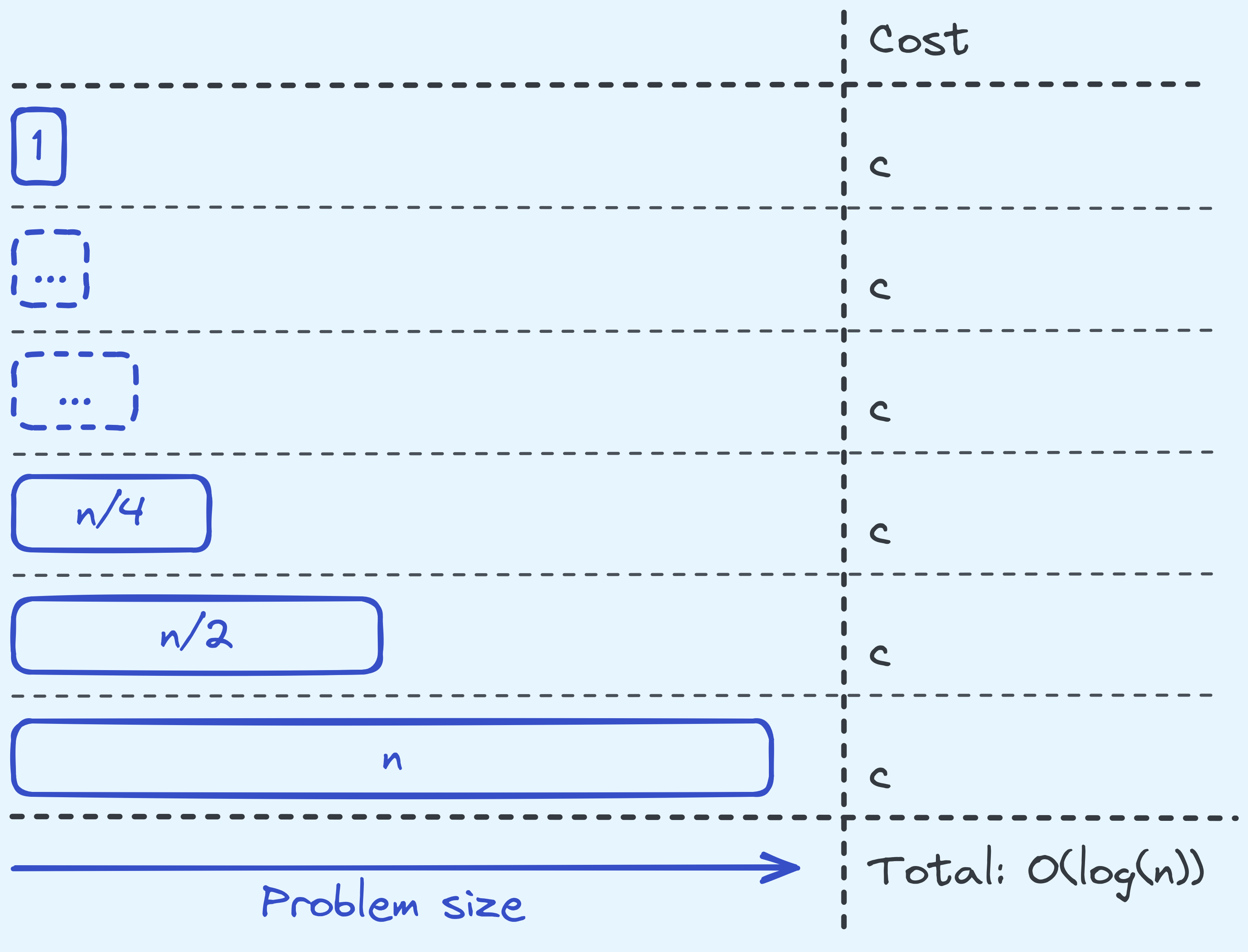
Analysing the time complexity of binary search.

So note here that at every level, we take \(c\) amount of steps (for some constant \(c\)) to do whatever we’re doing on the level itself (discounting the recursive calls). This is because we are only doing \(c\) many arithmetic operations, value copies, and comparisons of integers. Note here we are assuming that the comparisons cost \(c\) time. We will talk about when this assumption doesn’t hold much later in this post.

Next, there are \(O(\log(n))\) levels of recursion in total. To see this, note that when we start with a problem size of \(n\), in the next level the problem size we need to deal with is only half as large.

So in total, that is \(c \times O(\log(n))\) in time steps, or just \(O(\log(n))\).

What about factorial?

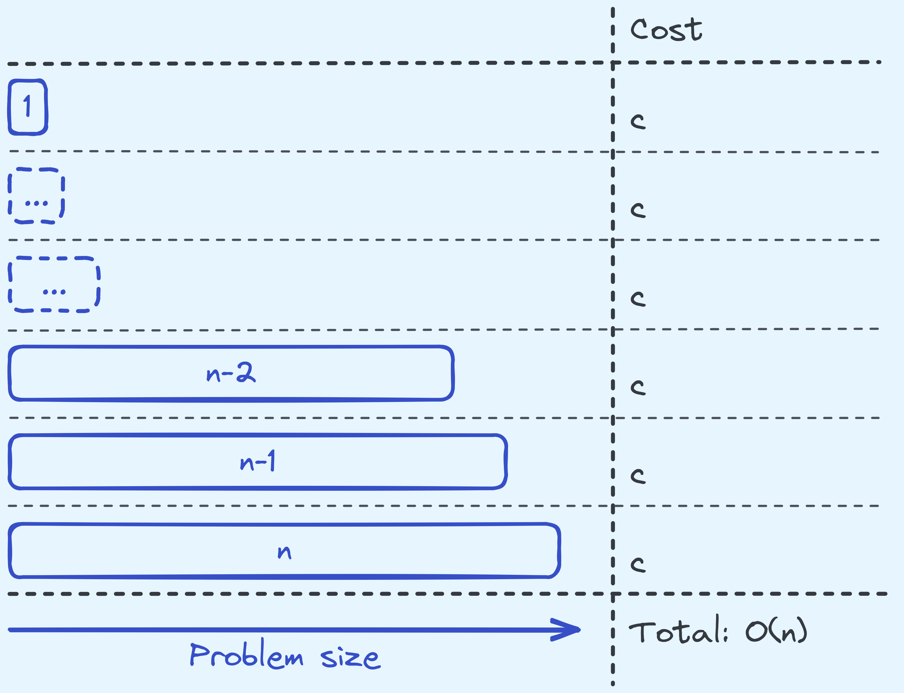
Analysing the time complexity of computing factorial.

It’s really similar, since at each level we’re just doing one comparison and one multiplication. So that costs \(c\) (for some constant \(c\)). Also there are \(O(n)\) levels of recursion, to see this, note that when starting with a problem size of \(n\), we recurse on a problem size of \(n-1\).

So in total, that is a cost of \(c \times O(n) = O(n)\).

You might have noticed I said constant \(c\), instead of \(O(1)\). The reason will be apparent in the next post. For now just trust that it’s important.

So one way of being able to figure out the time complexity, is to get the following:

1. The total work done at a given level of recursion, given a problem of size \(n\).
2. The total number of levels.

Then, summing those two up will give us what we want.

Now, the stair climbing problem is a little trickier, if you’ve never seen it before. The same trick that we want to do doesn’t seem quite to work here.

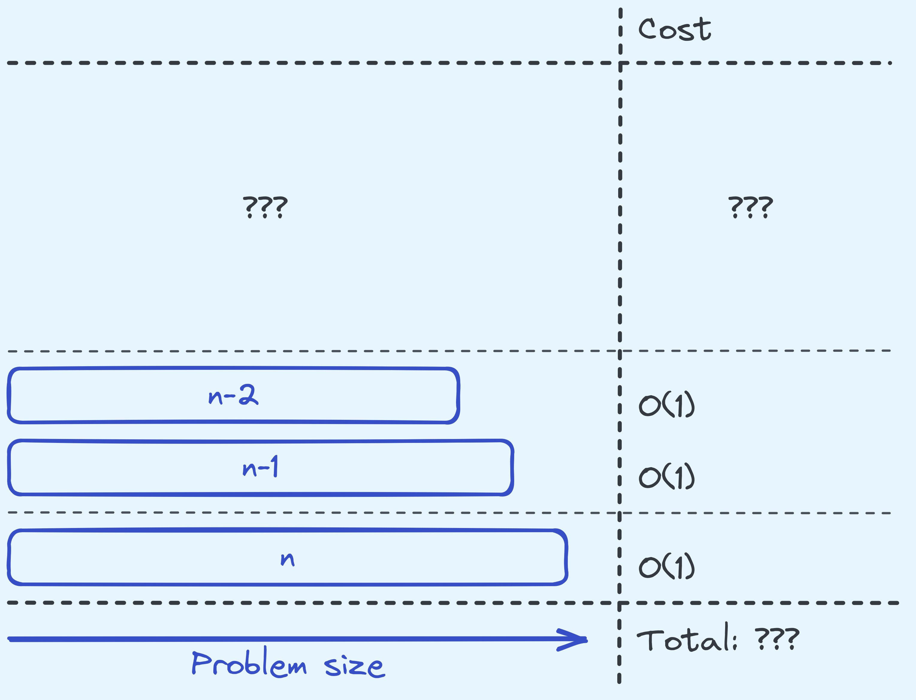
Analysing the time complexity of solving the stair climbing problem.

We know that at every level of the recursion we are only doing \(O(1)\) amount of work. But the difference is that, at least with the previous two algorithms, we know that each level was called exactly once. Over here, we don’t know how many times each level is called.

If you think about it, with a problem size of \(n\), it recurses on \(n-1\) and \(n-2\). And at the \(n-1\) level, it recurses on \(n-2\) and \(n-3\), and so on. This gets comlicated really quickly. Here’s an example with \(n = 5\):

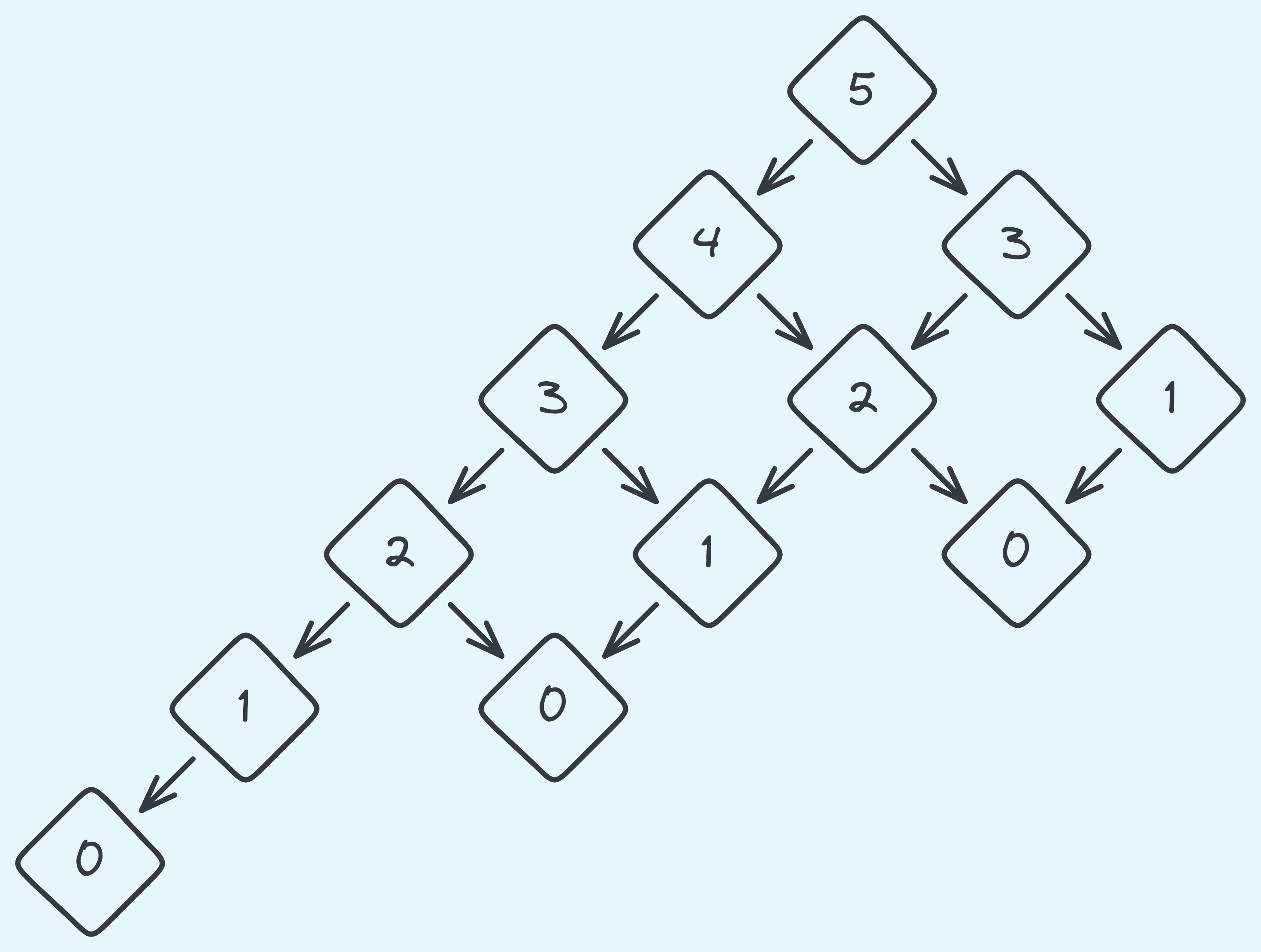
The recursion tree with \(n = 5\).

See how the “right” side of our recursion tree heads to \(1\) and \(0\) faster than the “left” side? Here’s how it looks like in general:

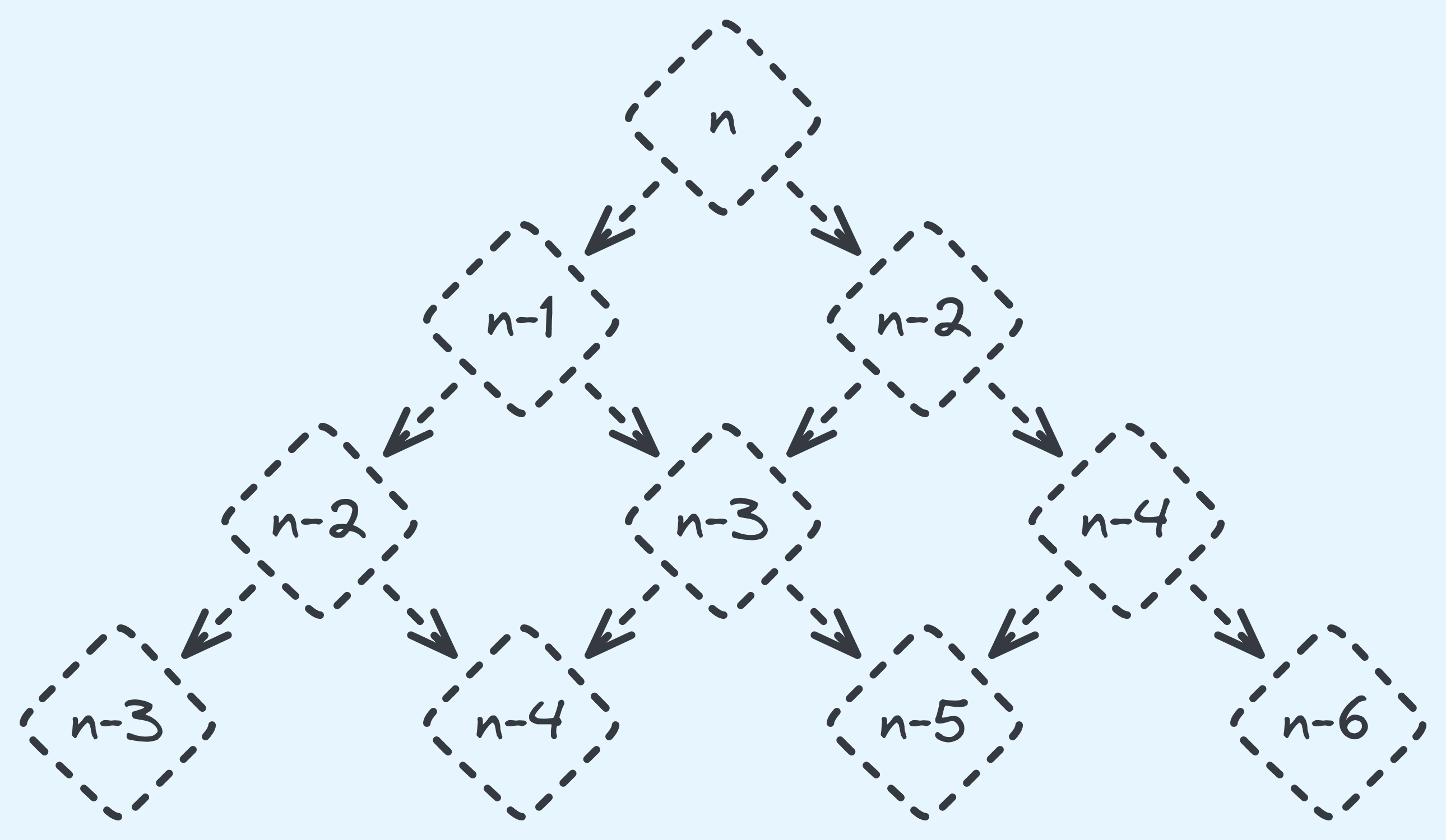
The recursion tree for general \(n\).

With this sort of recursion tree, it’s really hard to use the same tricks. So we’re going to use a different trick here. Introducing the time complexity function \(T(n)\)! It’s just a mathy name for “the total time steps for a problem of size \(n\)”. So for example, \(T(5)\) here should be \(12 \times c\), where \(c\) is the cost at each level of recursion. Now what the value of \(T(n)\)? \(T(n)\)’s value depends on \(T(n-1)\), and \(T(n-2)\). We also do constant work otherwise in our own level of recursion. So, mathematically:

\[T(n) = T(n - 1) + T(n - 2) + c\]

Okay, this might look reaaaally close to something you’ve seen before. ² But for the sake of simplicity, we’re going to do looser analysis that is easier for now. First, notice that \(T(n) = T(n - 1) + T(n - 2) + c \geq T(n) = T(n - 1) + c \geq T(n - 1)\).

So we can do the following:

\[\begin{aligned} T(n) &= T(n - 1) + T(n - 2) + c\\ &\leq T(n - 1) + T(n - 1) + c\\ &\leq 2 \cdot T(n - 1) + c \end{aligned}\]

We’ve replaced the \(T(n-2)\) with \(T(n-1)\). Now what we can do, is expand out \(T(n - 1)\) into being less than or equals to \(2 \cdot T(n - 2) + c\):

\[\begin{aligned} T(n) &\leq 2 \cdot T(n - 1) + c\\ &= 2 \left( 2 \cdot T(n - 2) + c \right) + c\\ &= 4 \cdot T(n - 2) + 2c + c\\ \end{aligned}\]

Now we can repeat this expansion, until \(T(0)\).

\[\begin{align} T(n) &\leq 4 \cdot T(n - 2) + 2c + c\\ &\leq 8 \cdot T(n - 3) + 4c + 2c + c\\ &\leq 16 \cdot T(n - 4) + 8c + 4c + 2c + c\\ &\leq 2^i \cdot T(n - i) + \sum_{j = 0}^{i - 1} 2^j \cdot c\\ &\leq 2^n \cdot T(0) + \sum_{j = 0}^{n - 1} 2^j \cdot c\\ &\leq 2^n \cdot T(0) + (2^n - 1) \cdot c\\ &\leq 2^n \cdot (T(0) + c) - c \end{align}\]

So our total cost has amounted to \(2^n \cdot (T(0) + c) - c\), and further note that \(T(0)\) should be some other constant \(c'\). So really it’s just a constant factor multiplied by \(2^n\). So our total cost is upper bounded by \(O(2^n)\).

What if this upper bound is too far away from the truth? Turns out it isn’t. But we’ll save that for a later date.

Don’t worry if time complexity analysis looks too complicated right now, we’re going to have a lot of practice doing this. What’s important is to just get a sense of how problems can be solved recursively.

A much more rigorous approach will be done after we’ve done more algorithms, so for now it’s more important that you work through what I’ve written here, and over time you’ll get a better sense of how to go about doing this.

Recursion Vs. Iteration

Let’s talk a little bit about whether we could implement some of these algorithms iteratively instead. That is to say, without any calls to itself.

In binary search, this is actually pretty straightforward, since there is nothing done in the recombination step, and everything is done in the decomposition, we can do this:

def binary_search(arr, query):
  low_index = 0
  high_index = len(arr) - 1
  while low_index <= high_index:
    middle_index = (low_index + high_index) // 2
    if query == arr[middle_index]:
      return True
    elif query < arr[middle_index]:
      high_index = middle_index - 1
    else:
      low_index = middle_index + 1
  return False

An iterative implementation of binary search.

This just looks a little more complicated to analyse. In fact, when we come around to formally proving correctness, proving the correctness of the recursive algorithm is going to go much smoother than the iterative one.

One thing that I want to talk about now though, isn’t the time complexity, because that is still the same. Instead, let’s compare the space complexity between the two.

Now for the iterative algorithm, this is easy to analyse. We’re just storing three more integers. So this is in \(O(1)\) space.

What about the space complexity of the recursive algorithm? You might be tempted to say \(O(1)\) since the iterative algorithm has demonstrated that.

But notice that every time we make a recursive call, we actually need to grow the stack a little. Since there are \(log_2(n)\) levels of recursion, and at each we store \(O(1)\) integers, the total space used is actually \(O(log(n))\). Yes, we don’t actually need to do that, and that’s why the the iterative algorithm can save space. So this is at least one of the reasons that I had mentioned earlier on about what happens when a function is called, this distinction is important because this is actually what happens in practice. (We’ll talk more about this in the context of real life recursion in a bit.)

Worse still, now that you know, think about what happens in the case of computing the factorial — it takes space \(O(n)\) when done recursively, when there’s a perfectly fine iterative algorithm that only takes \(O(1)\) space:

def factorial(n):
  value = 1
  while n > 0:
    value *= n
    n -= 1
  return value

An iterative implementation of the factorial algorithm.

The point is, sometimes recursive algorithms come naturally. But you have to bear in mind the potentially “hidden” costs of using a recursive algorithm.

Are iterative algorithms always better?

Not necessarily. Bear in mind that in practice, code always gets compiled down to something that is iterative. So really, if you ask me, you can start with something recursive at first then work on it and see if there’s potentially a better iterative solution. Sometimes there is, sometimes there isn’t. We’ll eventually see cases where there aren’t (known to be) any space savings.

Karatsuba’s Algorithm

We’ll end the main part of this post talking about Karatsuba’s algorithm. Here’s the problem that Karastsuba’s is trying to solve.

Stair Climbing:

Input: Given 2 numbers represented by a sequence of \(d\) bits a and b, i.e.:

1. a = a_d ... a_1 a_0
2. b = b_d ... b_1 b_0

Problem: Output the arithmetic product of a and b as a sequence of bits c.

Remember that I’ve briefly mentioned in the previous post on why multiplication should not be “free”, and basically the more digits you have, the more steps it should take to compute the product. So, let’s talk about one algorithm that does it decently quickly.

Also, just note that we can use the same algorithm to multiply two numbers with differing number of digits, just by padding the “smaller” number with leading zeroes. Also it’s going to be really convenient to take \(d\) as a power of \(2\). As it turns out, you only need to double the digits at most of any number to make it a power of \(2\).

The Basic Algorithm

Our starting point is formulating a basic algorithm that does things recursively. To see this, we’re going to start off with some math. We begin by expressing \(a\) and \(b\) as sums of their digits, and break this into two parts:

\[\begin{align} a &= \sum_{i = 0}^{d - 1} a_i \cdot 2^i \\ &= \left( \sum_{i = 0}^{ \frac{d}{2} - 1 } {a\ell}_i \cdot 2^i \right) + 2^{\frac{d}{2}} \left( \sum_{i = 0}^{ \frac{d}{2} - 1 } {ah}_i \cdot 2^i \right)\\ &= a\ell + 2^{\frac{d}{2}} \times ah \end{align}\]

You can think of \(a\ell\), as the lower bits of \(a\), and \(ah\) as the higher bits of \(a\). So now, if we did the same to \(b\):

\[\begin{align} a \times b &= \left( a\ell + 2^{\frac{d}{2}} \times ah \right) \times \left( b\ell + 2^{\frac{d}{2}} \times bh \right)\\ &= a\ell \times b\ell + 2^{\frac{d}{2}} \left( a\ell \times bh + b\ell \times ah \right) + 2^d \left( ah \times bh \right) \end{align}\]

Let’s break this down a little bit. If we can split up the numbers into two halves (each of \(d/2\) digits), we can compute the product by doing a few things:

1. Computing \(a\ell \times b\ell\), \(a\ell \times bh\), \(b\ell \times ah\), and \(ah \times bh\). (Recursion)
2. Shifting the some of the values by \(\frac{d}{2}\) digits. (Takes \(O(d)\) time.)
3. Shifting the some of the values by \(d\) digits. (Takes \(O(d)\) time.)
4. Addding the values together. (Takes \(O(d)\) time.)

Let’s see an implementation of this idea:

def shift(x, d):
  output_num_digits = len(x) + d
  output_digits = [0 for _ in range(len(output_num_digits))]

  for index in range(len(x)):
    output_digits[index + d] = x[index]
  return output_digits

def add(x, y):
  # we let x be the number with the longer digits
  # so if not, we swap x and y
  if len(y) > len(x):
    x, y = y, x

  # create our output array
  output_num_digits = max(len(x), len(y)) + 1
  output_digits = [0 for _ in range(len(output_num_digits))]

  carry_value = 0
  # iterate from the lowest significant digit 
  # up to the 2nd last of the output array
  for idx in range(len(output_num_digits) - 1):
    # if we are on the digit after `y`, then 
    # we just need to keep maintaining the carry value
    if idx >= len(y):
      output_digits[idx] = x[idx] | carry_value
      carry_value = x[idx] & carry_value

    # I'll be using the carry lookahead adder logic
    # don't worry too much about this, it's just 
    # adding 2 bits and a carry value
    else:
      output_digits[idx] = x[idx] ^ y[idx] ^ carry_value
      carry_value = ((x[idx] ^ y[idx]) & carry_value) | (x[idx] & y[idx])

  # the last carry bit into the last digit
  output_digits[-1] = carry_value
  return output_digits

def multiply(a, b):
  # get the number of digits
  num_digits = len(a)
  if num_digits == 1:
    return a[0] * b[0]

  # prepare al, and ah
  al = [], ah = []
  for index in range(num_digits // 2):
    al.append(a[index])
    ah.append(a[num_digits // 2 + index])
  
  # prepare bl, and bh
  bl = [], bh = []
  for index in range(num_digits // 2):
    bl.append(a[index])
    bh.append(a[num_digits // 2 + index])

  # compute the 4 products
  al_bl = multiply(al, bl)
  ah_bl = multiply(ah, bl)
  al_bh = multiply(al, bh)
  ah_bh = multiply(ah, bh)

  # add al_bh and ah_bl
  added_values = add(ah_bl, al_bh)

  # shift added_values by d//2 digits
  shifted_added_values = shift(added_values, num_digits//2)

  # shift ah_bh by d digits
  shifted_ah_bh = shift(ah_bh, num_digits)

  # add all the values up together
  return add(shifted_ah_bh, add(shifted_added_values, al_bl))
  

A basic recursive algorithm for multiplying two \(d\)-digit numbers.

Okay so let’s talk about how long this takes to run. Again, we’re going to let \(T(n)\) denote the time it takes to multiply two \(n\)-digit numbers. We make 4 recursive calls to multiply \(\frac{n}{2}\)-digit numbers. And then we take \(O(n)\) time to add some of the values up, and shift some of them. So for some positive constant \(c\), we can express the runtime in the following way:

\[\begin{aligned} T(n) &= 4 \cdot T(\frac{n}{2}) + cn && \text{}\\ &= 4 \left(4 T(\frac{n}{4}) + c\frac{n}{2} \right) + cn && \text{One round of expansion}\\ &= 4^2 \cdot T(\frac{n}{4}) + 2cn + cn && \text{Simplifying the terms}\\ &= 4^2 \left( 4 T(\frac{n}{8}) + c\frac{n}{4} \right) + 2cn + cn && \text{One round of expansion}\\ &= 4^3 \cdot T(\frac{n}{8}) + 4cn + 2cn + cn && \text{Simplifying the terms}\\ &\vdots\\ &= 4^{\log_{2}(n)} \cdot T(1) + \sum_{i = 0}^{\log_{2}(n) - 1} 2^i cn && \text{Generalising the sequence}\\ &= 4^{\log_{2}(n)} \cdot T(1) + cn \cdot 2^{\log_2(n)} && \\ &= n^{\log_{2}(4)} \cdot T(1) + c\cdot n^2 && \\ &= n^{2} \cdot T(1) + c\cdot n^2 && \\ \end{aligned}\]

Which works out to be \(O(n^2)\) time. Okay so that’s the baseline, how do we run faster? Notice in the math that a significant portion of the cost here is in how many recursive calls we’re making. Each time we do, the cost grows by a power of \(4\). So the leading idea right now is for us to work out the arithmetic so that we make less recursive calls.

Reducing the Number of Recursive Calls

Let’s go back to how we broke \(a\) and \(b\) into halves. See how during the multiplication we had three parts? \(ah \times bh\), \(a\ell \times bh + b\ell \times ah\), \(a\ell \times b\ell\). What if we could make the second part from the other two, along with some additions? Let’s see what happens with the following:

\[\begin{aligned} (a\ell + ah) \times (b\ell + bh) = a\ell \times b\ell + ah \times b\ell + a\ell \times bh + ah \times bh \end{aligned}\]

Turns out we get what we want, but added in are the terms \(ah \times bh\) and \(a\ell \times b\ell\), which we can figure out.

Then, with those three parts, we can do what we did before, shift the first part by \(2^n\), shift the middle part by \(2^{\frac{n}{2}}\), and sum up all three values and output that.

So this algorithm uses three multiplications, and a few more additions (and subtractions). So the sketch looks something like this:

def multiply(a, b):
  # get the number of digits
  num_digits = len(a)
  if num_digits == 1:
    return a[0] * b[0]

  # prepare al, and ah
  al = [], ah = []
  for index in range(num_digits // 2):
    al.append(a[index])
    ah.append(a[num_digits // 2 + index])
  
  # prepare bl, and bh
  bl = [], bh = []
  for index in range(num_digits // 2):
    bl.append(a[index])
    bh.append(a[num_digits // 2 + index])

  # compute the two parts
  al_bl = multiply(al, bl)
  ah_bh = multiply(ah, bh)

  # prepare the two added terms
  al_plus_ah = add(al, ah)
  bl_plus_bh = add(bl, bh)

  # prepare the special part
  middle_part = multiply(al_plus_ah, bl_plus_bh)

  # subtract the two other parts from the middle part
  middle_part = subtract(subtract(middle_part, al_bl), ah_bh)

  # shift added_values by d//2 digits
  shifted_added_values = shift(middle_part, num_digits//2)

  # shift ah_bh by d digits
  shifted_ah_bh = shift(ah_bh, num_digits)

  # add all the values up together
  return add(shifted_ah_bh, add(shifted_added_values, al_bl))
  

A sketch of Karatsuba’s Algorithm.

How does this algorithm compare then? We make \(3\) recursive calls on \(\frac{n}{2}\)-digit numbers and we take \(O(n)\) time to do everything else. Again, letting \(T(n)\) be our function for time complexity:

\[\begin{aligned} T(n) &= 3 \cdot T(\frac{n}{2}) + cn && \text{}\\ &= 3 \left(3 T(\frac{n}{2}) + c\cdot \frac{n}{2} \right) + cn && \text{One round of expansion}\\ &= 3^2 \cdot T(\frac{n}{2}) + 3c\cdot \frac{n}{2} + cn && \text{Simplifying the terms}\\ &= 3^2 \left(3 T(\frac{n}{4}) + c\cdot \frac{n}{4} \right) + 3c\frac{n}{2} + cn && \text{One round of expansion}\\ &= 3^3 \cdot T(\frac{n}{4}) + 3^2c \cdot \frac{n}{4} + 3c \cdot \frac{n}{2} + cn && \text{Simplifying the terms} & \vdots\\ &= 3^{\log_2(n)} \cdot T(1) + \sum_{i = 0}^{\log_2(n) - 1} \left(\frac{3}{2}\right)^i cn && \text{Generalising the sequence}\\ &= 3^{\log_2(n)} \cdot T(1) + \left( \frac{3}{2} \right)^{\log_2(n)} cn && \text{Geometric sum}\\ &= n^{\log_2(3)} \cdot T(1) + n^{\log_2(\frac{3}{2})} \cdot cn && \\ &= n^{\log_2(3)} \cdot T(1) + cn^{\log_2(3)} && \end{aligned}\]

Which works out to be \(O(n^{\log_2(3)}) \approx O(n^{1.585})\). So plotting that out on a graph, we get:

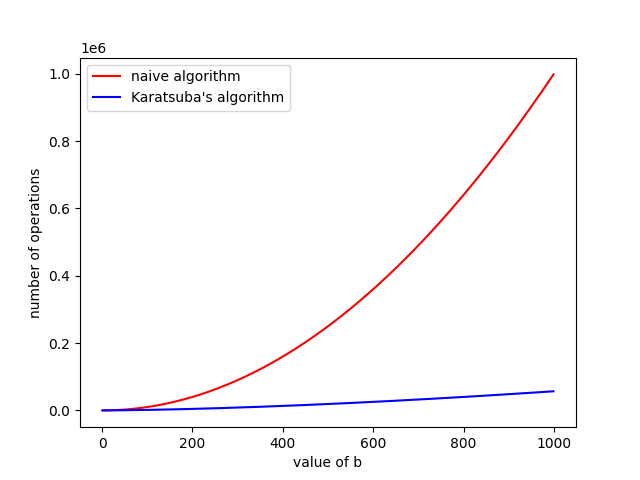
Time Complexity of Naive vs. Karatsuba.

Bear in mind that we’re just graphing the asymptotic functions and we’ve not put in any constants. So the actual runtimes might look different.

---

Some Random Notes About Recursion In Practice

So this part of the post is mostly bonus content. But I think these details are worth mentioning, and rarely mentioned in a course on algorithms course. We’ll talk about optimisations that happen in real life, along with some other real life use cases that make use of some of the stuff I’ve mentioned here.

Tail Call Optimisation

Let’s talk a little bit about what assembly comes out when we implement something recursive. In particular, let’s talk a little more in detail about the space usage of a recursive implementation of an algorithm vs. an iterative implementaiton.

We’ll begin with the binary search algorithm, and we’ll use C++. For reference, here’s the code that I’m compiling:

#include <stddef.h>
#include <vector>

bool binary_search(size_t left, size_t right, std::vector<int> &list, int query){
    if(right > left){
        return false;
    }

    size_t mid = (left + right) / 2;
    if(list[mid] == query){
        return true;
    }

    if(query < list[mid]){
        return binary_search(left, mid - 1, list, query);
    }

    if(query > list[mid]){
        return binary_search(mid + 1, right, list, query);
    }
}

Some C++ code for implementing binary search.

What about the x86 that is emitted? Now g++ has a few optimisation settings. First let’s see what happens on -O0. Which has little to no optimisations.

binary_search(unsigned long, unsigned long, std::vector<int, std::allocator<int> >&, int):
        push    rbp
        mov     rbp, rsp
        sub     rsp, 48
        mov     QWORD PTR [rbp-24], rdi
        mov     QWORD PTR [rbp-32], rsi
        mov     QWORD PTR [rbp-40], rdx
        mov     DWORD PTR [rbp-44], ecx
        mov     rax, QWORD PTR [rbp-32]
        cmp     QWORD PTR [rbp-24], rax
        jnb     .L2
        mov     eax, 0
        jmp     .L1
.L2:
        mov     rdx, QWORD PTR [rbp-24]
        mov     rax, QWORD PTR [rbp-32]
        add     rax, rdx
        shr     rax
        mov     QWORD PTR [rbp-8], rax
        mov     rdx, QWORD PTR [rbp-8]
        mov     rax, QWORD PTR [rbp-40]
        mov     rsi, rdx
        mov     rdi, rax
        call    std::vector<int, std::allocator<int> >::operator[](unsigned long)
        mov     eax, DWORD PTR [rax]
        cmp     DWORD PTR [rbp-44], eax
        sete    al
        test    al, al
        je      .L4
        mov     eax, 1
        jmp     .L1
.L4:
        mov     rdx, QWORD PTR [rbp-8]
        mov     rax, QWORD PTR [rbp-40]
        mov     rsi, rdx
        mov     rdi, rax
        call    std::vector<int, std::allocator<int> >::operator[](unsigned long)
        mov     eax, DWORD PTR [rax]
        cmp     DWORD PTR [rbp-44], eax
        setl    al
        test    al, al
        je      .L5
        mov     rax, QWORD PTR [rbp-8]
        lea     rsi, [rax-1]
        mov     ecx, DWORD PTR [rbp-44]
        mov     rdx, QWORD PTR [rbp-40]
        mov     rax, QWORD PTR [rbp-24]
        mov     rdi, rax
        call    binary_search(unsigned long, unsigned long, std::vector<int, std::allocator<int> >&, int)
        jmp     .L1
.L5:
        mov     rdx, QWORD PTR [rbp-8]
        mov     rax, QWORD PTR [rbp-40]
        mov     rsi, rdx
        mov     rdi, rax
        call    std::vector<int, std::allocator<int> >::operator[](unsigned long)
        mov     eax, DWORD PTR [rax]
        cmp     DWORD PTR [rbp-44], eax
        setg    al
        test    al, al
        je      .L6
        mov     rax, QWORD PTR [rbp-8]
        lea     rdi, [rax+1]
        mov     ecx, DWORD PTR [rbp-44]
        mov     rdx, QWORD PTR [rbp-40]
        mov     rax, QWORD PTR [rbp-32]
        mov     rsi, rax
        call    binary_search(unsigned long, unsigned long, std::vector<int, std::allocator<int> >&, int)
        jmp     .L1
.L6:
.L1:
        leave
        ret

Output from x86-64 gcc 12.2.0 on -O0 -std=c++20.

Now there’s a lot to read here, so I’ll save your time. I just want you to focus on the fact that there are call instructions on lines 49 and 68. And right after those lines, you can see that we’re going to jmp to line 71 which basically does a leave and a ret. Essentially, the point is right after our function call, we’re going to immediately return without operating on any of the other values in our stack frame.

The second thing I want you to note is that whenever binary_search is called, we need to allocate more space on the stack. You can spot that on line 4, when the stack pointer is reduced. Then, lines 5 to 8 move the arguments we need into the stack frame.

Alright, so this means that if our recursion depth is \(5\), then we need to make \(5\) stack frames for binary_search, and so on. In general since the recursion depth is \(O(\log(n))\) at most, the space usage is \(O(\log(n))\).

But as I’ve mentioned, we know a much simpler iterative algorithm that doesn’t actually need to take up so much space. Can the compiler make the same observation for this case? Let’s try compiling with -O3 instead.

binary_search(unsigned long, unsigned long, std::vector<int, std::allocator<int> >&, int):
        cmp     rdi, rsi
        jb      .L8
        mov     rdx, QWORD PTR [rdx]
.L3:
        lea     rax, [rsi+rdi]
        shr     rax
        cmp     DWORD PTR [rdx+rax*4], ecx
        je      .L7
.L11:
        jle     .L4
        lea     rsi, [rax-1]
        cmp     rdi, rsi
        jnb     .L3
.L8:
        xor     eax, eax
        ret
.L4:
        lea     rdi, [rax+1]
        cmp     rdi, rsi
        jb      .L8
        lea     rax, [rsi+rdi]
        shr     rax
        cmp     DWORD PTR [rdx+rax*4], ecx
        jne     .L11
.L7:
        mov     eax, 1
        ret

Output from x86-64 gcc 12.2.0 on -O3 -std=c++20.

Well look at that, no more calls! In fact this is really just the iterative solution I had written earlier on.

So this is part of what’s called tail call optimisation. ³ Let’s talk about that. Semantically, a tail call is the call is to a function that is at the end of a function.

def main_function(input):
  func_1(input)
  func_2(input)
  if func_3(input):
    return func_4(input)
  elif func_5(input):
    return func_6(input)
  else:
    return 7
  return func_7(input)

So in the example above, func_4 and func_6 are tail calls because it’s the last call before a function. Note here func_7 is not a tail call even though it’s at the “end” of the function definition, because it will never be called.

The point is that for something like binary search, where we can express the algorithm with only tail calls, we don’t actually need to make more stack frames, we can just use the current stack frame that we’re on.

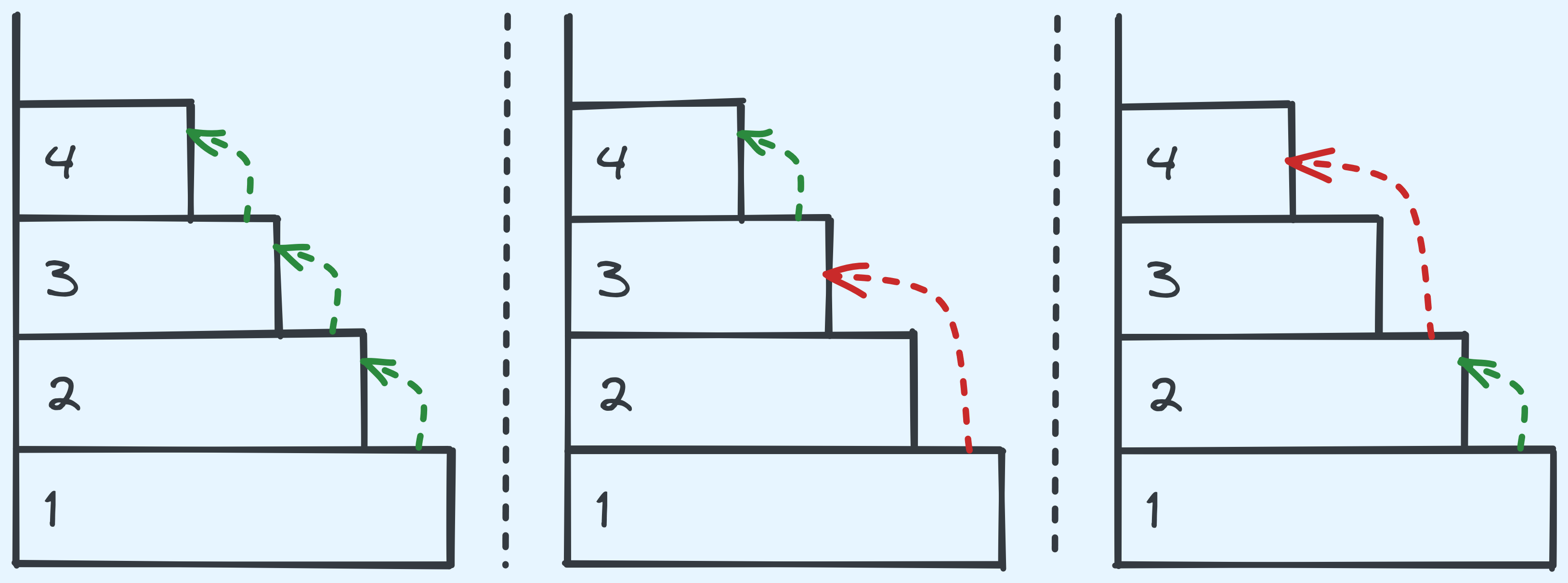
Why’s that? because whatever we did in our current level of recursion, know for a fact we don’t need any of it after the next call is done. Let’s compare having TCO without TCO with some diagrams in case that helps. We’ll do a simple one, and let’s say that in the binary search we are doing, we recurse to the left once and we need to return True after that.

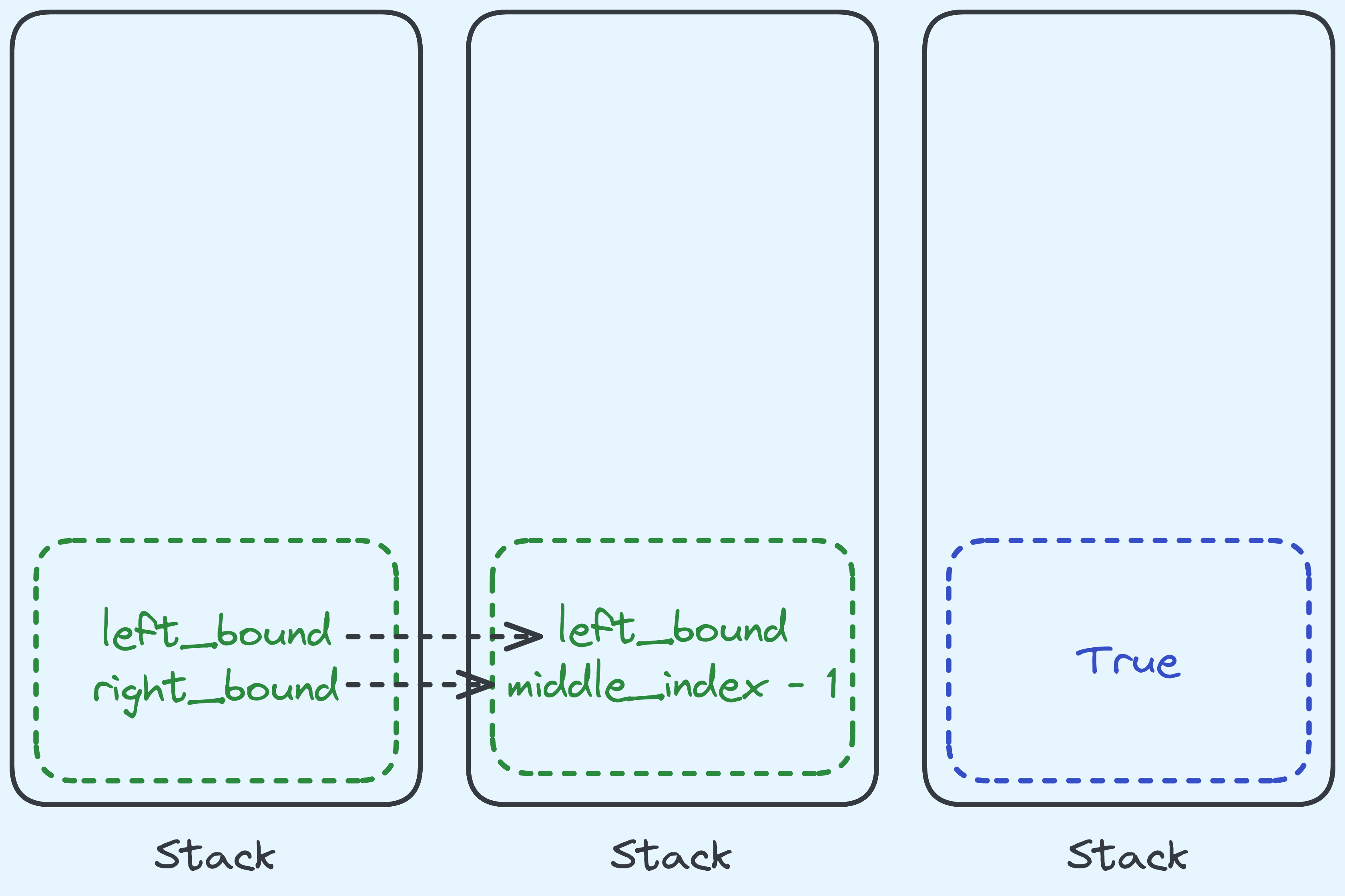
What happens in binary search without TCO.

Without tail call optimisation, we would have to move (among other) arguments, left_bound and middle_index - 1 to the next stack frame. Then when that call has a result, we’re just forwarding it along. We don’t use any of the data that we had kept before the call. Any tail call enjoys very similar behaviour. So because of that, instead of making a new stack frame, we can just replace the current one with the required arguments. Like so:

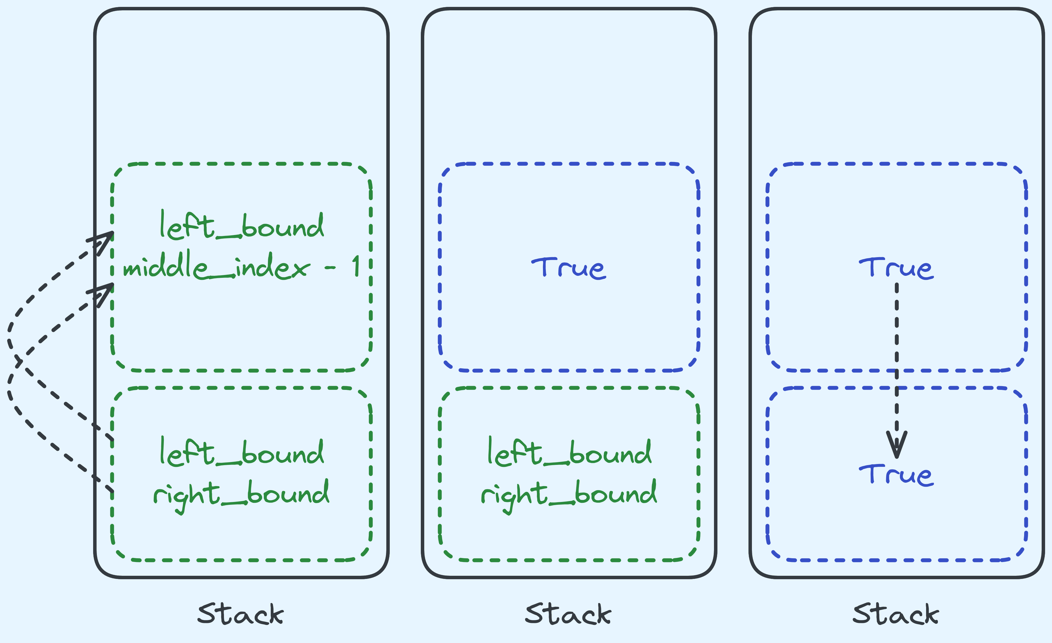
What happens in binary search with TCO.

In fact, we don’t really have to move anything, we can just keep them in the same place and trust the next level of recursion to just pick up where we left of. If you look at the instructions emitted when using -O3 you’ll see that indeed we don’t move the arguments between loop iterations.

What about factorial? Is that a tail call?

Actually, it isn’t! Because we need to wait for the result of the call, then we need to operate on the result. Like so:

Computing factorial actually operates on the result of the call.

But let’s just see what sort of x86 gets emitted between -O0 vs -O3. For reference, here’s the C++ I’ve written:

#include <stdint.h>

uint64_t factorial(uint64_t n){
    if(n == 0){
        return 1;
    }
    return n * factorial(n - 1);
}

Some C++ code for implementing factorial.

And here’s the emitted x86 on -O0:

factorial(unsigned long):
        push    rbp
        mov     rbp, rsp
        sub     rsp, 16
        mov     QWORD PTR [rbp-8], rdi
        cmp     QWORD PTR [rbp-8], 0
        jne     .L2
        mov     eax, 1
        jmp     .L3
.L2:
        mov     rax, QWORD PTR [rbp-8]
        sub     rax, 1
        mov     rdi, rax
        call    factorial(unsigned long)
        imul    rax, QWORD PTR [rbp-8]
.L3:
        leave
        ret

Okay so far, this looks like what we think it would look like. There’s a call on line 14, and we can see the stack frame being made and the sole argument being moved in on lines 4 and 5. Okay, what about on -O3?

factorial(unsigned long):
        mov     eax, 1
        test    rdi, rdi
        je      .L1
.L2:
        imul    rax, rdi
        sub     rdi, 1
        jne     .L2
.L1:
        ret

Output from x86-64 gcc 12.2.0 on -O3 -std=c++20.

For some reason, g++ knows how to optimise this into a simple loop. I don’t really have an explanation for this right now. I might look more into what they’re doing in the future but for now just know that there are nice optimisations that work beyond just tail calls.

How Does Binary Search Measure Up In Practice?

I’m making a separate post (which I will link here subsequently on talking about this).

Git Bisect

If you use git you might have heard of git-bisect. Let’s talk a little bit about what it does, and why binary search is useful. ⁴

As a brief introduction, git tracks the changes made source code (among other things) and basically stores it in the form of a graph. So, something like this:

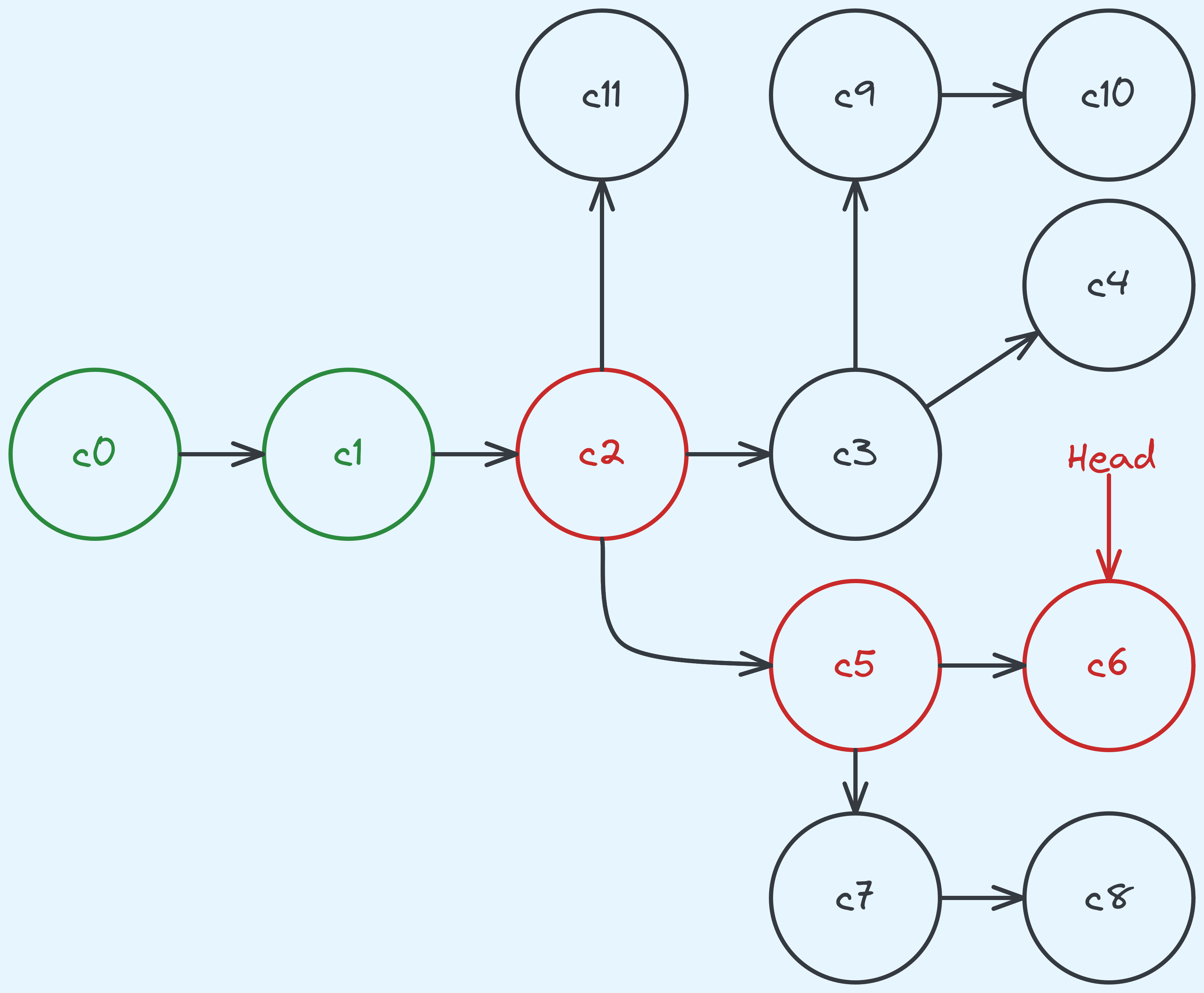
A graph keeping track of the different versions of the source code.

Think of each node (which we will call a commit) as a version. So c1 preceeds c2, which preceeds both c3 and c5 and so on. What happens if let’s say you’re on c6 and you realise that there’s a bug in the code? There’s a chance that this issue has always been present and you might now need to “go back in time” to find out what was the change that introduced the bug.

So one thing we could do is test all the commits up that line of the history, which includes c0, c1, c2, c5, c6. Now one interesting thing about the structure of the graph is that we can’t “randomly access” commits, it takes linear time to check out a commit. (Not without first traversing the history and putting them into an array. But that already takes linear time.) And yet, git bisect would binary search on this history by first getting us to test the middle commit, and if we find out that is is broken, we move further back in the history, otherwise further forward.

Why? It already takes linear time anyway, so what’s the point? The cool thing is that visiting a specific commit (or version) doesn’t actually take that long. The significantly bigger cost is in building the code, and then running the tests (especially for larger projects). Because of that, what we want to minimise, is the time spent on building and testing, which is essentialy a “comparison” in this binary search. When seen in this light, it becomes a little more apparent why binary search is favoured here — the algorithm inherently minimises comparisons!

There are a few more details about complicated situations where git bisect might actually take a lot of “comparisons” but I’m not going to go into that. ⁵

---

Solution: Tower of Hanoi

We’re going to generalise the algorithm a little bit. We are going to build solutions that take in \(n\) disks, and a source location \(s\), and a target location \(t\). So to solve the exercise, we need to move \(n\) disks from \(1\) to \(3\).

The first big observation we make is that in order to move the largest disk, the \(n - 1\) disks need to be in location \(2\), so that we can move disk \(n\) from location \(1\) to location \(3\). Then we need to move the \(n - 1\) disks from location \(2\) to location \(3\). But hey! Moving the \(n-1\) disks is just a smaller problem. Also note that we can happily do whatever we want when moving only the \(n-1\) disks while pretending the \(n^{th}\) disk doesn’t exist since they are all narrower.

In general, if we want to move from some location \(s\) to some location \(t\), note that \(1 + 2 + 3 = 6\), so \(6 - s - t\) just gives us a “middle” location which we use to store the intermediate stack of \(n - 1\) disks.

One last observation that we should make is that when only moving a single disk (which is our base case), it we should be able to “just” move it.

So the algorithm looks like this:

def tower_of_hanoi(num_disks, source_location, target_location):
  if num_disks == 1:
    print(F"move disk of width 1 from {source_location} to {target_location}")
    return

  # a way of gettting the "middle" location
  mid_location = 6 - source_location - target_location

  tower_of_hanoi(num_disks - 1, source_location, mid_location)
  print(F"move disk of width {num_disks} from {source_location} to {target_location}")
  tower_of_hanoi(num_disks - 1, mid_location, target_location)
  return 

---

Thanks

Thanks to Christian for helping to give this post a looksee.

---

1. We will see in the future this can be a little arbitrary, but for now it’s not a major concern. We will just very reasonable base cases. ↩

2. It almost looks like Fibonacci. ↩

3. I think a strict definition of “tail call” does not admit computing the factorial. But the optimisation does kick in for basically the same reason. ↩

4. Thanks to Christian Welly for mentioning this idea to me! ↩

5. Some extra goodies about git bisect: (1) Linus Torvald’s Discussion and (2) a theoretical analysis of git bisect ↩